Fitting the I part is easy we simply difference d times. The same observation applies to seasonal multiplicative model. Thus to fit an ARIMA(p,d,q) model to X you compute Y =(I-B)d X (shortening your data set by d observations) and then you fit an ARMA(p,q) model to Y. So we assume that d=0.
Simplest case: fitting the AR(1) model
Our basic strategy will be:
Generally the full likelihood is rather complicated; we will use conditional likelihoods and ad hoc estimates of some parameters to simplify the situation.
If the errors ![]() are normal then so is the series X. In general
the vector
are normal then so is the series X. In general
the vector
![]() has a
has a
![]() where
where
![]() and
and ![]() is a vector all of whose entries are
is a vector all of whose entries are
![]() .
The joint density of X is
.
The joint density of X is

It is possible to carry out full maximum likelihood by maximizing the quantity in question numerically. In general this is hard, however.
Here I indicate some standard tactics. In your homework I will be asking you to carry through this analysis for one particular model.
Consider the model
![\begin{displaymath}\ell(\mu,\rho,\sigma) = - \frac{1}{2\sigma^2}\sum_1^{T-1} \le...
...-\rho(x_{k-1}-\mu)\right]^2
-(T-1)\log(\sigma) + \log(f_{X_0})
\end{displaymath}](img17.gif)


+ (1-\rho^2)(x_0-\mu)\right\}
\end{displaymath}](img22.gif)


Now compute
![\begin{displaymath}\frac{\partial}{\partial\sigma} \ell = \frac{1}{\sigma^3}\lef...
...\mu)\right]^2 +(1-\rho^2)(x_0-\mu)^2\right\}
-\frac{T}{\sigma}
\end{displaymath}](img27.gif)
![\begin{displaymath}\hat\sigma^2(\rho) = \frac{\left\{
\sum_1^{T-1}\left[x_k-\mu(...
...-\mu(\rho))\right]^2
+(1-\rho^2)(x_0-\mu(\rho))^2\right\}}{T}
\end{displaymath}](img28.gif)
To find ![]() you now plug
you now plug
![]() and
and
![]() into
into ![]() (getting the so called profile likelihood
(getting the so called profile likelihood
![]() )
and maximize over
)
and maximize over ![]() .
Having thus found
.
Having thus found ![]() the mles of
the mles of ![]() and
and
![]() are simply
are simply
![]() and
and
![]() .
.
It is worth observing that fitted residuals can then be calculated:
In general, we simplify the maximum likelihood problem several ways:
In the AR(1) case Y is just
![]() while
Z is X0. We take our conditional log-likelihood to be
while
Z is X0. We take our conditional log-likelihood to be
![\begin{align*}\ell(\mu,\rho,\sigma) & = \sum_1^{T-1} \log(f_{X_t\vert X_0,\ldots...
...{T-1} \left[X_t-\mu -
\rho(X_{t-1}-\mu)\right]^2 -(T-1)\log(\sigma)
\end{align*}](img46.gif)
![\begin{displaymath}\ell(\bar{X},\rho,\sigma) = \frac{-1}{2\sigma^2} \sum_1^{T-1}...
..._t-\bar{X} - \rho(X_{t-1}-\bar{X})\right]^2 -(T-1)\log(\sigma)
\end{displaymath}](img47.gif)

![\begin{displaymath}\hat\sigma^2 = \frac{ \sum_1^{T-1}
\left[X_t-\bar{X} - \hat\rho(X_{t-1}-\bar{X})\right]^2}{T-1}
\end{displaymath}](img49.gif)

Notice that we have made a great many suggestions for simplifications and adjustments. This is typical of statistical research - many ideas, only slightly different from each other, are suggested and compared. In practice it seems likely that there is very little difference between all the methods. I am asking you in a homework problem to investigate the differences between several of these methods on a single data set.
For the model

![\begin{displaymath}\ell_c(\phi,\mu,\sigma) = -\frac{1}{2\sigma^2}
\sum_p^{T-1} \...
...-\mu - \sum_1^p a_i(X_{t-i} - \mu)\right]^2
-(T-p)\log(\sigma)
\end{displaymath}](img54.gif)
![\begin{displaymath}-\frac{1}{2\sigma^2}
\sum_p^{T-1} \left[ X_t-\bar{X} - \sum_1^p a_i(X_{t-i} - \bar{X})\right]^2
-(T-p)\log(\sigma)
\end{displaymath}](img56.gif)
![\begin{displaymath}\sum_p^{T-1} \hat\epsilon_t^2 = \sum_p^{T-1} \left[ X_t-\bar{X} - \sum_1^p
a_i(X_{t-i} - \bar{X})\right]^2
\end{displaymath}](img58.gif)
![\begin{displaymath}\left[\begin{array}{c} X_p -\bar{X} \\ \vdots \\ X_{T-1} -\bar{X} \end{array} \right]
\end{displaymath}](img59.gif)
![\begin{displaymath}\left[\begin{array}{ccc}
X_{p-1} -\bar{X}& \cdots & X_0 -\bar...
...{T-2} -\bar{X}& \cdots & X_{T-p-1} -\bar{X}
\end{array}\right]
\end{displaymath}](img60.gif)
An alternative to estimating ![]() by
by ![]() is to define
is to define
![]() and then recognize that
and then recognize that
![\begin{displaymath}\ell(\alpha,\phi,\sigma) = -\frac{1}{2\sigma^2}
\sum_p^{T-1} ...
...[ X_t-\alpha - \sum_1^p a_iX_{t-i}\right]^2
-(T-p)\log(\sigma)
\end{displaymath}](img62.gif)
![\begin{displaymath}\left[\begin{array}{c} X_p \\ \vdots \\ X_{T-1} \end{array} \right]
\end{displaymath}](img63.gif)
![\begin{displaymath}\left[\begin{array}{ccc}
X_{p-1} & \cdots & X_0
\\
\vdots &...
... & \vdots
\\
X_{T-2} & \cdots & X_{T-p-1}
\end{array}\right]
\end{displaymath}](img64.gif)
Notice that if we put
![\begin{displaymath}Z=\left[\begin{array}{ccc}
X_{p-1} -\bar{X}& \cdots & X_0 -\b...
...{T-2} -\bar{X}& \cdots & X_{T-p-1} -\bar{X}
\end{array}\right]
\end{displaymath}](img68.gif)
![\begin{displaymath}Z^tZ \approx T \left[\begin{array}{cccc}
\hat{C}(0) & \hat{C}...
...
\cdots & \cdots & \hat{C}(1) & \hat{C}(0)
\end{array}\right]
\end{displaymath}](img69.gif)
![\begin{displaymath}Y=\left[\begin{array}{c} X_p -\bar{X} \\ \vdots \\ X_{T-1} -\bar{X}
\end{array} \right]
\end{displaymath}](img70.gif)
![\begin{displaymath}Z^tY \approx T \left[\begin{array}{c} \hat{C}(1) \\ \vdots \\ \hat{C}(p)
\end{array}\right]
\end{displaymath}](img71.gif)
To compute a full mle of
![]() you generally begin by finding preliminary estimates
you generally begin by finding preliminary estimates
![]() say by one of the conditional likelihood
methods above and then iterate via Newton-Raphson or
some other scheme for numerical maximization of the
log-likelihood.
say by one of the conditional likelihood
methods above and then iterate via Newton-Raphson or
some other scheme for numerical maximization of the
log-likelihood.
Here we consider the model with known mean (generally this
will mean we estimate
![]() and subtract the mean
from all the observations):
and subtract the mean
from all the observations):
In general X has a
![]() distribution and, letting
distribution and, letting
![]() denote the vector of bis we find
denote the vector of bis we find
![\begin{displaymath}\Sigma = \left[\begin{array}{ccccc}
\sigma^2(1+b_1^2) & -b_1\...
... & \cdots & -b_1\sigma^2& \sigma^2(1+b_1^2)
\end{array}\right]
\end{displaymath}](img79.gif)
Notice that

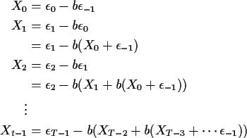
Now imagine that the data were actually

![\begin{align*}\ell(b,\sigma) = &
\frac{-\epsilon_{-1}}{2\sigma^2} - \log(\sigma)...
...2 X_{t-2} - \cdots -\psi^{t+1} \epsilon_{-1})^2+\log(\sigma)\right]
\end{align*}](img84.gif)
Method A: Put
![]() since 0 is
the most probable value and maximize
since 0 is
the most probable value and maximize
![\begin{displaymath}-T\log(\sigma) - \frac{1}{2\sigma^2} \sum_0^{T-1} \left[X_t - \psi X_{t-1}
- \psi^2 X_{t-2} - \cdots -\psi^{t}X_0\right]^2
\end{displaymath}](img86.gif)
Method B: Backcasting is the process of
guessing
![]() on the basis of the data; we replace
on the basis of the data; we replace
![]() in the log likelihood by
in the log likelihood by
We will use the EM algorithm to solve this problem.