Postscript version of these notes

STAT 804: Notes on Lecture 9

Fitting higher order autoregressions

For the model

$$X_t- \mu = \sum_1^p a_i(X_{t-1}-\mu) + \epsilon_t$$

we will use conditional likelihood again. Let $\phi$ denote the vector $(a_1,\ldots, a_p)^t$. Now we condition on the first p values of X and use

$$\ell_c(\phi,\mu,\sigma) = -\frac{1}{2\sigma^2} \sum_p^{T-1} \... ...-\mu - \sum_1^p a_i(X_{t-i} - \mu)\right]^2 -(T-p)\log(\sigma)$$

If we estimate $\mu$ using $\bar{X}$ we find that we are trying to maximize

$$-\frac{1}{2\sigma^2} \sum_p^{T-1} \left[ X_t-\bar{X} - \sum_1^p a_i(X_{t-i} - \bar{X})\right]^2 -(T-p)\log(\sigma)$$

To estimate $a_1,\ldots,a_p$ then we merely minimize the sum of squares

$$\sum_p^{T-1} \hat\epsilon_t^2 = \sum_p^{T-1} \left[ X_t-\bar{X} - \sum_1^p a_i(X_{t-i} - \bar{X})\right]^2$$

This is a straightforward regression problem. We regress the response vector

$$\left[\begin{array}{c} X_p -\bar{X} \\ \vdots \\ X_{T-1} -\bar{X} \end{array} \right]$$

on the design matrix

$$\left[\begin{array}{ccc} X_{p-1} -\bar{X}& \cdots & X_0 -\bar... ...{T-2} -\bar{X}& \cdots & X_{T-p-1} -\bar{X} \end{array}\right]$$

An alternative to estimating $\mu$ by $\bar{X}$ is to define $\alpha = \mu(1-\sum a_i)$ and then recognize that

$$\ell(\alpha,\phi,\sigma) = -\frac{1}{2\sigma^2} \sum_p^{T-1} ... ...[ X_t-\alpha - \sum_1^p a_iX_{t-i}\right]^2 -(T-p)\log(\sigma)$$

is maximized by regressing the vector

$$\left[\begin{array}{c} X_p \\ \vdots \\ X_{T-1} \end{array} \right]$$

on the design matrix

$$\left[\begin{array}{ccc} X_{p-1} & \cdots & X_0 \\ \vdots &... ... & \vdots \\ X_{T-2} & \cdots & X_{T-p-1} \end{array}\right]$$

From $\hat\alpha$ and $\hat\phi$ we would get an estimate for $\mu$ by

$$\hat\mu = \frac{\hat\alpha}{1-\sum \hat{a}_i}$$

Notice that if we put

$$Z=\left[\begin{array}{ccc} X_{p-1} -\bar{X}& \cdots & X_0 -\b... ...{T-2} -\bar{X}& \cdots & X_{T-p-1} -\bar{X} \end{array}\right]$$

then

$$Z^tZ \approx T \left[\begin{array}{cccc} \hat{C}(0) & \hat{C}... ... \cdots & \cdots & \hat{C}(1) & \hat{C}(0) \end{array}\right]$$

and if

$$Y=\left[\begin{array}{c} X_p -\bar{X} \\ \vdots \\ X_{T-1} -\bar{X} \end{array} \right]$$

then

$$Z^tY \approx T \left[\begin{array}{c} \hat{C}(1) \\ \vdots \\ \hat{C}(p) \end{array}\right]$$

so that the normal equations (from least squares)

$$Z^t Z \phi = Z^T Y$$

are nearly the Yule-Walker equations again.

Full maximum likelihood

To compute a full mle of $\theta=(\mu,\phi,\sigma)$you generally begin by finding preliminary estimates $\hat\theta$ say by one of the conditional likelihood methods above and then iterate via Newton-Raphson or some other scheme for numerical maximization of the log-likelihood.

Fitting MA(q) models

Here we consider the model with known mean (generally this will mean we estimate $\hat\mu=\bar{X}$ and subtract the mean from all the observations):

$$X_t = \epsilon_t - b_1 \epsilon_{t-1} - \cdots - b_q\epsilon_{t-q}$$

In general X has a $MVN(0,\Sigma)$ distribution and, letting $\psi$ denote the vector of b_is we find

$$\ell(\psi,\sigma) = -\frac{1}{2}\left[\log(\det(\Sigma)) - X^T \Sigma^{-1} X\right]$$

Here X denotes the column vector of all the data. As an example consider q=1 so that

$$\Sigma = \left[\begin{array}{ccccc} \sigma^2(1+b_1^2) & -b_1\... ... & \cdots & -b_1\sigma^2& \sigma^2(1+b_1^2) \end{array}\right]$$

It is not so easy to work with the determinant and inverse of matrices like this. Instead we try to mimic the conditional inference approach above but with a twist; we now condition on something we haven't observed -- $\epsilon_{-1}$.

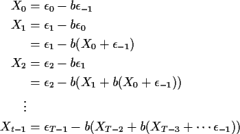
Notice that
$$\begin{align*}X_0 & = \epsilon_0 - b\epsilon_{-1} \\ X_1 & = \epsilon_1 - b\eps... ... = \epsilon_{T-1} - b(X_{T-2} + b (X_{T-3} + \cdots \epsilon_{-1})) \end{align*}$$
Now imagine that the data were actually

$$\epsilon_{-1}, X_0,\ldots,X_{T-1}$$

Then the same idea we used for an AR(1) would give
$$\begin{align*}\ell(b,\sigma) & = \log(f(\epsilon_{-1},\sigma)) + \log(f(X_0,\ldo... ..._0^{T-1} \log(f(X_t\vert X_{t-1},\ldots,X_0,\epsilon_{-1},b,\sigma) \end{align*}$$
The parameters are listed in the conditions in this formula merely to indicate which terms depend on which parameters. For Gaussian $\epsilon$s the terms in this likelihood are squares as usual (plus logarithms of $\sigma$) leading to
$$\begin{align*}\ell(b,\sigma) = & \frac{-\epsilon_{-1}}{2\sigma^2} - \log(\sigma)... ...2 X_{t-2} - \cdots -\psi^{t+1} \epsilon_{-1})^2+\log(\sigma)\right] \end{align*}$$
We will estimate the parameters by maximizing this function after getting rid of $\epsilon_{-1}$ somehow.

Method A: Put $\epsilon_{-1}=0$ since 0 is the most probable value and maximize

$$-T\log(\sigma) - \frac{1}{2\sigma^2} \sum_0^{T-1} \left[X_t - \psi X_{t-1} - \psi^2 X_{t-2} - \cdots -\psi^{t}X_0\right]^2$$

Notice that for large T the coefficients of $\epsilon_{-1}$ are close to 0 for most t and the remaining few terms are negligible relatively to the total.

Method B: Backcasting is the process of guessing $\epsilon_{-1}$ on the basis of the data; we replace $\epsilon_{-1}$ in the log likelihood by

$$\text{E}(\epsilon_{-1}\vert X_0,\ldots,X_{T-1})\, .$$

The problem is that this quantity depends on b and $\sigma$.

We will use the EM algorithm to solve this problem. The algorithm can be applied when we have (real or imaginary) missing data. Suppose the data we have is X; some other data we didn't get is Y and Z=(X,Y). It often happens that we can think of a Y we didn't observe in such a way that the likelihood for the whole data set Z would be simple. In that case we can try to maximize the likelihood for X by following a two step algorithm first discussed in detail by Dempster, Laid and Rubin. This algorithm has two steps:

1.

The E or Estimation step. We ``estimate'' the missing data Y by computing $\text{E}(Y\vert X)$. Technically, we are supposed to estimate the likelihood function based on Z. Factor the density of Z as

f_Z = f_Y|Xf_X

and take logs to get

$$\ell(\theta\vert Z) = \log(f_{Y\vert X}) + \ell(\theta\vert X)$$

We actually estimate the log conditional density (which is a function of $\theta$) by computing

$$\text{E}_{\theta_0}(\log(f_{Y\vert X})\vert X)$$

Notice the subscript $\theta_0$ on $\text{E}$. This indicates that you have to know the parameter to compute the conditional expectation. Notice too that there is another $\theta$ in the conditional expectation - the log conditional density has a parameter in it.

2.

We then maximize our estimate of $\ell(\theta\vert Z)$ to get a new value $\theta_1$ for $\theta$. Go back to step 1 with this $\theta_1$ replacing $\theta_0$ and iterate.

To get started we need a preliminary estimate. Now look at our problem. In our case the quantity Y is $\epsilon_{-1}$. Rather than work with the log-likelihood directly we work with Y. Our preliminary estimate of Y is 0. We use this value to estimate $\theta$ as above getting an estimate $\theta_0$. Then we compute $\text{E}_{\theta_0}(\epsilon_{-1}\vert X)$ and replace $\epsilon_{-1}$ in the log-likelihood above by this conditional expectation. Then iterate. This process of guessing $\epsilon_{-1}$ is called backcasting.

Summary

• The log likelihood based on $\epsilon_{-1},X_0,\ldots,X_{T-1}$is
  
  $$\frac{-\epsilon_{-1}^2}{2\sigma^2} -(T+1) \log(\sigma) - \fra... ..._{t-1} - \psi^2 X_{t-2} - \cdots -\psi^{t+1} \epsilon_{-1})^2$$
  
  

• Put $\epsilon_{-1}=0$ in this formula and estimate $\psi$ by minimizing
  
  $$\sum\hat\epsilon_t^2$$
  
  
  where
  
  $$\hat\epsilon_t = X_t - \psi X_{t-1} - \psi^2 X_{t-2} - \cdots -\psi^t X_0$$
  
  
  for $t=0,\ldots,T-1$.

• Now compute $\text{E}(\epsilon_{-1}\vert X_0,\ldots,X_{T-1})$Box, Jenkins and Reinsel presents an algorithm to do so based on the fact that there are actually two MA representations of corresponding to a given covariance function (the invertible one and a non-invertible one). The non-invertible representation is
  
  $$X_t = e_t + \frac{1}{\psi} e_{t+1};$$
  
  
  this form can be used to carry out the computation of the conditional expection.

• Iterate, re-estimating $\psi$ and recomputing the backcast value of $\epsilon_{-1}$ if needed.