

Postscript version of these notes
STAT 350: Lecture 16
Reading: There is no really relevant part of the text.
Theory of F and t tests
Independence: If
 are random
variables then we call
 independent if
for any sets
 .
.
We usually either:
- Assume independence because there is no physical way for the value of
any of the random variables to influence any of the others.
OR
- We prove independence.
How do we prove independence? We use the notion of a joint density.
We say
 have joint density function
 if
if
We are interested here in joint densities because independence of
 is equivalent to
for some densities
 .
In this case fi is the density
of Ui.
[ ASIDE: notice that for an independent sample the joint density
is the likelihood function!]
Application to Normals: Standard Case
If
then the joint density of Z, denoted
 is
is
where
So
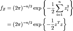
where
Application to Normals: General Case
If  and A is invertible then for any set
  we have

Make the change of variables  in this integral to get
where
J(x) denotes the Jacobian of the transformation
Algebraic manipulation of the integral then gives
where
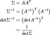
The conclusion of this algebra is that the
 density is
What if A is not invertible? Ans: there is no density.
How do we apply this density?
Suppose
and
If
 then
then
- 1.
-

- 2.
- In the homework you will verify that
- 3.
- Writing
and
we find
- 4.
- So, if
 and
and
 we see that

so that X1 and X2 are independent.
Summary: If
![${\rm Cov}(X_1,X_2) = {\rm E}[(X_1-\mu_1)(X_2-\mu_2)^T]=0$](img37.gif) then X1 is
independent of X2.
then X1 is
independent of X2.
Warning: This only works provided
Fact: However, it works even if  is singular, but
you can't prove it as easily using densities.
Application:
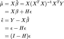
So
Hence
Now
so
![\begin{align*}AA^T & = \sigma^2 \left[
\begin{array}{c} H \\ \hline I-H \end{arr...
...sigma^2 \left[ \begin{array}{cc} H & 0
\\ 0 & I-H\end{array}\right]
\end{align*}](img44.gif)
The 0s prove that
 and
and  are
independent. It follows that
 ,
the regression
sum of squares (not adjusted) is independent of
 ,
the Error sum of squares.
Joint Densities
Suppose Z1 and Z2 are independent standard normals. In class I said
that their joint density was
Here I want to show you the meaning of joint density by computing the
density of a  random variable.
Let
U = Z12+Z22. By definition U has a  distribution with 2
degrees of freedom. The cumulative distribution function of U
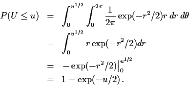
is
For  this is 0 so take
  .
The event that
  is the same as the event that the point
(Z1,Z2) is in the circle centered at the origin and having
radius u1/2, that is, if A is the circle of this radius
then
By definition of density this is a double integral
You do this integral in polar co-ordinates. Letting
 and
and
 we see that
The Jacobian of the transformation is r so that
 becomes
 .
Finally the region of integration is simply
 and
and
 so that
The density of U can be found by differentiating to get
which is the exponential density with mean 2. This means that the
 density is really an exponential density.


Richard Lockhart
1999-01-13
![]() are random
variables then we call
are random
variables then we call
![]() independent if
independent if
![]() have joint density function
have joint density function
![]() if
if

![\begin{displaymath}Z = \left[ \begin{array}{c} Z_1 \\ \vdots \\ Z_n\end{array} \right]
\sim MVN(0,I_{n \times n})
\end{displaymath}](img10.gif)


![\begin{displaymath}z=\left[ \begin{array}{c} z_1 \\ \vdots \\ z_n \end{array} \right]
\end{displaymath}](img15.gif)
![]() and A is invertible then for any set
and A is invertible then for any set ![]() we have
we have

![]() in this integral to get
in this integral to get


![\begin{displaymath}X = \left[\begin{array}{c} X_1 \\ \hline X_2 \end{array}\right]
\end{displaymath}](img26.gif)
![\begin{displaymath}\Sigma = \left[\begin{array}{c\vert c} \Sigma_{11} & \Sigma_{12}
\\
\hline
\Sigma_{21} & \Sigma_{22} \end{array}\right]
\end{displaymath}](img27.gif)
![]() then
then
![\begin{displaymath}\Sigma^{-1} = \left[\begin{array}{c\vert c} \Sigma^{-1}_{11} & 0
\\
\hline
0 & \Sigma^{-1}_{22} \end{array}\right]
\end{displaymath}](img30.gif)
![\begin{displaymath}x = \left[ \begin{array}{c} x_1 \\ \hline x_2 \end{array} \right]
\end{displaymath}](img31.gif)
![\begin{displaymath}\mu = \left[ \begin{array}{c} \mu_1 \\ \hline \mu_2 \end{array} \right]
\end{displaymath}](img32.gif)

![]() then X1 is
independent of X2.
then X1 is
independent of X2.
![\begin{displaymath}X = \left[\begin{array}{c} X_1 \\ \hline X_2 \end{array}\right] \sim
MVN(\mu,\Sigma)
\end{displaymath}](img38.gif)
![]() is singular, but
you can't prove it as easily using densities.
is singular, but
you can't prove it as easily using densities.

![\begin{displaymath}\left[
\begin{array}{c} \hat\mu \\ \hline \hat\epsilon \end{a...
...
\left[
\begin{array}{c} \mu \\ \hline 0 \end{array}\right]}_b
\end{displaymath}](img41.gif)
![\begin{displaymath}\left[
\begin{array}{c} \hat\mu \\ \hline \hat\epsilon \end{a...
...begin{array}{c} \mu \\ \hline 0 \end{array}\right];AA^T\right)
\end{displaymath}](img42.gif)
![\begin{displaymath}A = \sigma\left[
\begin{array}{c} H \\ \hline I-H \end{array}\right]
\end{displaymath}](img43.gif)
![\begin{align*}AA^T & = \sigma^2 \left[
\begin{array}{c} H \\ \hline I-H \end{arr...
...sigma^2 \left[ \begin{array}{cc} H & 0
\\ 0 & I-H\end{array}\right]
\end{align*}](img44.gif)
![]() distribution with 2
degrees of freedom. The cumulative distribution function of U
is
distribution with 2
degrees of freedom. The cumulative distribution function of U
is

