Postscript version of these notes

STAT 350: Lecture 15

Reading: Chapter 7 sections 1, 2. Chpater 5 sections 11 and 12.

Extra Sum of Squares

Here is a more general version of the extra Sum of Squares method. Consider two $n \times p$ design matrices, X and X^*. Suppose that there is a $p \times p$ invertible matrix A such that X=X^* A.

If we fit the model $Y=X\beta+\epsilon$ we get
$$\begin{align*}\hat\beta & = (X^T X)^{-1} X^T Y \\ \hat\mu &= X\hat\beta = X(X^T X)^{-1} X^T Y \end{align*}$$
Fitting the model $Y=X^* \beta^* + \epsilon$ we get
$$\begin{align*}\hat\beta^* & = ({X^*}^T X^*)^{-1} {X^*}^T Y \\ \hat\mu^* &= X^*\hat\beta^* = X^*({X^*}^T X^*)^{-1} {X^*}^T Y \end{align*}$$

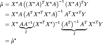
Now plug in X^* A for X in $\hat\beta$ and $\hat\mu$ to get
$$\begin{align*}\hat\mu & = X^* A \left( (X^* A)^T X^* A\right)^{-1} (X^* A)^T Y \... ...underbrace{\left(A^T\right)^{-1}A^T}_{I} {X^*}^TY \\ & = \hat\mu^* \end{align*}$$
So X and X^* lead to the same fitted vector.

Notice that $\beta^* = A\beta$ and $\hat\beta^* = A\hat\beta$.

If X=X^*A for some invertible A then

$${\rm col}(X) = {\rm col}(X^*)$$

Now suppose that X=X^*A but that A is not invertible (for example X might have fewer columns than X^*). The idea is that in this case X describes a sub-model of that described by X.

Example: The two sample problem.

$$X^* = \left[ \begin{array}{cc} 1 & 0 \\ 1 & 0 \\ \vdots &... ... 0 \\ 0 & 1 \\ \vdots & \vdots \\ 0 & 1 \end{array}\right]$$

where there are n₁ rows of $[1 \quad 0]$ and n₂ of $[0 \quad 1]$.

$$X=\left[ \begin{array}{c} 1 \\ \vdots \\ 1 \end{array}\right]$$

where X is $(n_1+n_2) \times 1$. Then

$$X^* \left[\begin{array}{c} 1 \\ 1 \end{array}\right] = X$$

The model

$$Y = X^* \beta + \epsilon$$

is really
$$\begin{align*}Y_i & = \beta_1 + \epsilon_i \qquad 1 \le 1 \le n_1 \\ Y_i & = \beta_2 + \epsilon_i \qquad n_1+1 \le i \le n_1+n_2 \end{align*}$$
that is, it is the model for two samples of sizes n₁ and n₂ with means $\beta_1$ and $\beta_2$. The model

$$Y=X\beta_1+\epsilon$$

is just

$$Y_i = \beta_1 + \epsilon_i$$

that is, that the Y_i are an iid sample from a single population.

We compare these two models to test $H_o: \beta_1 = \beta_2$ using

$$F = \frac{({\rm ESS}_R - {\rm ESS}_F)/1}{ {\rm ESS}_F/(n_1+n_2 - 2)} = \left( \mbox{2 sample $t$}\right)^2$$

Summary: to compare two models with design matrices X and X^* we need

$${\rm col}(X) \subset {\rm col}(X^*) \qquad {\rm col}(X) \neq {\rm col}(X^*)$$

That is, we need the restricted model to be a special case of the full model where we put some linear combinations of the $\beta$s equal to constants. (The constants are usually 0.)

In our example consider the special case n₁ = n₂. If we reparametrize the * model using

$$\mu=\frac{\beta_1+\beta_2}{2} \qquad \alpha = \beta_1 - \mu$$

then we find

$$X^*\beta = X^{**} \left[ \begin{array}{c} \mu \\ \alpha \end{array} \right]$$

where

$$X^{**} = \left[ \begin{array}{cc} 1 & 1 \\ 1 & 1 \\ \vdot... ...\\ 1 & -1 \\ \vdots & \vdots \\ 1 & -1 \end{array} \right]$$

In this case we see that X is a submatrix of X^**. This is why the extra sum of squares principle can be used whenever the restricted model is a special case of the full model, even if X is not a submatrix of X^*.

Another Extra Sum of Squares Example: two way layout

We have data Y_i,j,k for i from 1 to I, j from 1 to J and k from 1 to K where i labels the row effect, j labels the column effect and k labels the replicate. When K is more than 1 we generally check for interactions by comparing the additive model

$$Y_{i,j,k} = \mu + \alpha_i + \beta_j + \epsilon_{i,j,k}$$

to a saturated model in which the mean $\mu_{i,j}$ for the combination i,j is unrestricted. Thus the full model is

$$Y_{i,j,k} = \mu_{i,j}j + \epsilon_{i,j,k} \, .$$

The additive model is not identifiable (that is, the design matrix is not of full rank) unless some conditions are imposed on the row effects $\alpha_i$ and the column effects $\beta_j$. A common restriction imposed is that the effects sum to 0; this restriction is then used to eliminate $\alpha_I$ and $\beta_J$ from the model equations. The resulting design matrix then has 1+(I-1)+(J-1) = I+J-1 columns and looks like

$$X_{\mbox{add}} = \left[\begin{array}{rrrcrrr} 1 & 1 & 0 & \cd... ...\ 1 & -1 & -1 & \cdots & -1 & -1 & \cdots \end{array}\right]$$

(There are K copies of the first row for the observations in population i=1,j=1, then K copies of the row for observations in population i=1,j=2 and so on till we get to j=J. Elimination of $\beta_J = -\beta_1 -\beta_2 -\cdots - \beta_{J-1}$ produces -1's in the J-1 columns corresponding to the $\beta$'s. Then we move to the JK rows corresponding to i=2 and so on with the last JK rows having -1's in the $\alpha$ columns reflecting the identity $\alpha_I = - \alpha_1 -\cdots - \alpha_{I-1}$.)

The full model is often reparametrized as

$$Y_{i,j,k} = \mu + \alpha_i + \beta_j + \lambda_{i,j} + \epsilon_{i,j,k}$$

but the design matrix is actually much simpler for the first parameterization:

$$X_{\mbox{Full}} = \left[\begin{array}{rrrrr} 1 & 0 & 0 & \cd... ...\\ & & \vdots \\ 0 & 0 & 0 & \cdots & 1 \end{array}\right]$$

where there are K copies of the first row, $[1,0,\ldots,0]$ and then K copies of $[0,1,0,\ldots,0]$ and so on. There are a total of IJ columns and IJK rows.

It is not hard to find a matrix A such that

$$X_{\mbox{add}} = X_{\mbox{Full}} A$$

For instance the first column of A will be all 1's since this corresponds to adding the columns of $X_{\mbox{Full}}$ together and this produces a column of 1's which is the first column of $X_{\mbox{add}}$. To produce the second column of $X_{\mbox{add}}$ we have to add together the first I columns of $X_{\mbox{Full}}$ and then subtract out the last I columns of $X_{\mbox{Full}}$. Thus the second column of A consists of I 1's followed by I(J-2) 0's followed by I -1's.