Postscript version of these notes

STAT 350: Lecture 5

Some Examples

Polynomial Regression

We consider data on average claims paid per policy for automobile insurance in New Brunswick in the years 1971-1980:

Year	1971	1972	1973	1974	1975	1976	1977	1978	1979	1980
Cost	45.13	51.71	60.17	64.83	65.24	65.17	67.65	79.80	96.13	115.19

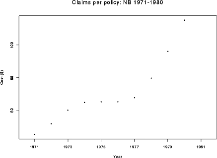
Here is a plot of the data:

One goal of analysis is to extrapolate the Costs for 2.25 years beyond the end of the data; this should help the insurance company set premiums.

In this example we fit polynomials of degrees from 1 to 5, plot the fits, compute error sums of squares and examine the 5 resulting extrapolations to the year 1982.25.

The model equation for a pth degree polynomial is

$$Y_i = \beta_0 + \beta_1 t_i + \cdots + \beta_p t_i^p + \epsilon_i$$

where the t_i are the covariate values (the dates in the example). Notice:

• p+1 parameters (sometimes there will be p parameters in total and sometimes a total of p+1 - the intercept plus p others)

• $\beta_0$ is the intercept

The design matrix is given by

$$X = \left[ \begin{array}{cccc} 1 & t_1 & \cdots & t_1^p \\ 1... ...cdots & \vdots \\ 1 & t_n & \cdots & t_n^p \end{array}\right]$$

Goals of Analysis:

• estimate $\beta$s

• select good value of p. This presents a trade-off:

  • large p fits data better BUT

  • small p is easier to interpret.

In the following you will see the SAS analyses of the data, though I have edited the analyses severely.

Using SAS the following code will fit the model for a degree five polynomial.

options pagesize=60 linesize=80;
data insure;
  infile 'insure.dat';
  input year cost;
  code = year - 1975.5 ;
  c2=code**2 ;
  c3=code**3 ;
  c4=code**4 ;
  c5=code**5 ;
proc glm  data=insure;
   model cost = code c2 c3 c4 c5 ;
run ;

NOTE: the computation of code is important. The software has great difficulty with the calculation without the subtraction. It should seem reasonable that there is no harm in counting years with 1975.5 taken to be the 0 point of the variable time.

Here is some edited output:

Dependent Variable: COST
                                     Sum of            Mean
Source                  DF          Squares          Square   F Value     Pr > F

Model                    5     3935.2507732     787.0501546   2147.50     0.0001

Error                    4        1.4659868       0.3664967

Corrected Total          9     3936.7167600


Source                  DF        Type I SS     Mean Square   F Value     Pr > F

CODE                     1     3328.3209709    3328.3209709   9081.45     0.0001
C2                       1      298.6522917     298.6522917    814.88     0.0001
C3                       1      278.9323940     278.9323940    761.08     0.0001
C4                       1        0.0006756       0.0006756      0.00     0.9678
C5                       1       29.3444412      29.3444412     80.07     0.0009

From these sums of squares I can compute error sums of squares for each of the five models.

Degree	Error Sum of Squares
1	608.395789
2	309.743498
3	30.811104
4	30.810428
5	1.465987

In this table the last line is produced directly by SAS. Each higher line consists of the sum of the line below together with the Type I SS figure from SAS. So, for instance, the ESS for a degree 4 fit is just the ESS for a degree 5 fit plus 29.3444412, the ESS for a degree 3 fit is the ESS for a degree 2 fit plus 0.006756, and so on.

The actual estimates of the coefficients must be obtained by running SAS proc glm 5 times, once for each model. The fitted models are
$$\begin{align*}y & = 71.102+6.3516 t\\ y & = 64.897+6.3516 t + 0.7521 t^2\\ y &... ... & = 64.888 -0.5024t +0.7562 t^2+ 0.8016 t^3 -0.0002 t^4 -0.0194t^5 \end{align*}$$
You should observe that sometimes, but not always, adding a term to the model changes coefficients of terms already in the model. These lead to the following predictions for 1982.25:

Degree	$\hat\mu_{1982.25}$
1	113.98
2	142.04
3	204.74
4	204.50
5	70.26

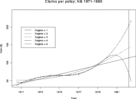
Here is a plot of the five resulting fitted polynomials, superimposed on the data and extended to 1983.

I have added a vertical line at 1982.25 so that you can see that the different fits give wildly different extrapolated values. You will not be able to see a difference between the degree 3 and degree 4 fits. Overall the degree 3 fit is probably best but does have a lot of parameters for the number of data points. The degree 5 fit is a statistically significant improvement over the degree 3 and 4 fits. But it is hard to believe in the polynomial model outside the range of the data! Extrapolation is very dangerous and unreliable.