Postscript version of these notes

STAT 804

Lecture 23 Notes

Estimating the spectrum

We now consider the quality of $\vert{\hat X}\vert^2$ as an estimate of f_X. We have already shown that

$${\rm E}(\vert{\hat X}\vert^2) \to f_X(\omega) \, .$$

However we will see that the variance of this estimate $\hat f$ of f does not go to 0 so that the estimate is not consistent.

It is easier technically to consider the case of a normal mean 0 process X. For normal data the real and imaginary parts of $\hat X$ have normal distributions. Both have mean 0. The variances are

$$\frac{1}{T} \sum_{r=0}^{T-1}\sum_{s=0}^{T-1} \cos(2\pi\omega r)\cos(2\pi\omega s) C_X(r-s)$$

and

$$\frac{1}{T} \sum_{r=0}^{T-1}\sum_{s=0}^{T-1} \sin(2\pi\omega r)\sin(2\pi\omega s) C_X(r-s)$$

while the covariance between the real and imaginary parts is

$$\frac{1}{T} \sum_{r=0}^{T-1}\sum_{s=0}^{T-1} \cos(2\pi\omega r)\sin(2\pi\omega s) C_X(r-s) \, .$$

Consider as an example the covariance, and use the usual complex exponential identities to write the covariance as

$$\frac{1}{4T} \sum_{r=0}^{T-1}\sum_{s=0}^{T-1} C_X(r-s)(e^{2\p... ...e^{-2\pi\omega ri})(e^{2\pi\omega si}-e^{-2\pi\omega si}) \, .$$

Now make the change of variables u=r-s and v=r+s in the double sum. The variable u runs from -(T-1) to T-1 while when u is fixed the possible values of v run, for u positive from u to 2(T-1)-u by increments of 2 and, for u negative from -u to 2(T-1)+u by increments of 2. For each value of u there are then T-|u| possible values of vand the covariance becomes

$$\frac{1}{4T} \sum_{u=-(T-1)}^{T-1} \sum_{v=\vert u\vert,v\mbo... ...pi\omega vi} +e^{-2\pi\omega u} -e^{2\pi\omega u}\right\} \, .$$

The last two terms, involving u only, are

$$\frac{1}{4T} \sum_{u=-(T-1)}^{T-1} (T-\vert u\vert)C_X(u) (e^{-2\pi\omega u} -e^{2\pi\omega u})$$

The terms u and -u cancel each other while the term with u=0 is 0 itself so that this term is 0.

The terms above involving v may be simplified by using geometric series to do the inside sums over v. The result is a coefficient of C(u)which is bounded (bounded by $4/(1-\cos(2\pi\omega))$ for instance. Then since

$$\frac{1}{4T} \sum_{u=-(T-1)}^{T-1}C_X(u) \to 0$$

we have checked that the covariance between the real and imaginary parts of ${\hat X}(\omega)$ converges to 0 as $T\to\infty$.

Our previous calculations of the expectation of $\vert{\hat X}(\omega)\vert^2$can be mimicked to show that the two variances each converge to $f_X(\omega)/2$. It follows that the vector $\sqrt{2/f(\omega)}(Real({\hat X}(\omega)), Im({\hat X}(\omega)))$ converges to a bivariate standard normal. The squared length of this vector then converges in distribution to the squared length of a standard bivariate normal which is exactly $\chi^2_2$ or exponential with mean 2.

Summary: $\vert{\hat X}\vert(\omega)^2$ converges in distribution to an exponential random variable with mean $f(\omega)$. In particular, $\vert{\hat X}\vert(\omega)^2$ is not a consistent estimator of $f(\omega)$.

Improved estimates

To get better estimates we need either to resort to parametric estimation techniques or do some smoothing. We will look at the latter idea first. If $f(\omega)$ is smooth in the neighbourhood of some $\omega_0$ then we can take estimates of $f(\omega)$ at a number of points nearby to $\omega_0$ and average them somehow. Averaging will reduce the variance though it will introduce bias usually because the things being averaged all have different expected values.

The simplest kind of estimator is a moving average - we define

$${\hat f}(k/T) = \frac{1}{2L+1} \sum_{\ell = -L}^L \vert{\hat X}((k+\ell)/T)\vert^2$$

It turns out that the quantities being averaged are asymptotically independent so that the estimate has the same distribution as an average of 2L+1 exponentials which is just a chi-squared with L+2 degrees of freedom multiplied by $f(\omega_0)/(4L+2)$. It is possible then to produce a consistent estimate by letting L grow slowly with T but we won't investigate this rather mathematical problem carefully here.

Other weighted averages are possible; several are implemented in the S-Plus function spectrum. Here are some points to note about this estimation problem:

• Each estimate $\vert{\hat X}(k/T)\vert^2$ has expected value $f(k/T)+{\rm Bias}_T(k/T)$ where a (complicated) formula for the bias can be deduced from the algebra above. The expected value of an estimate of the form
  
  $$\sum_{\ell = -L}^L w_\ell \vert{\hat X}((k+\ell)/T)\vert^2$$
  
  
  is then
  
  $$\sum_{\ell = -L}^L w_\ell f((k+\ell)/T) + \sum_{\ell = -L}^L w_\ell{\rm Bias}_T((k+\ell)/T)$$
  
  
  If f is roughly linear around k/T then the first term will be quite close to f(k/T) when the weights make the estimate an average, that is, they sum to 1. However, this approximation will be poor in the neighbourhood of any peak in the spectrum which will be flattened by this averaging. The second term in the expectation, on the other hand, has no particular reason to average out to 0; increasing L without dealing with this bias will eventually be fruitless as the bias becomes the dominant component in the error. A common tactic to dealing with this bias is tapering, where we compute
  
  $${\hat X}^*(\omega) = \sum h\left(\frac{t}{T}\right)X_t \exp(2\pi\omega ti)$$
  
  
  and use as a periodogram
  
  $$\frac{\vert{\hat X}^*(\omega)\vert^2}{\sum h^2\left(\frac{t}{T}\right)}$$
  
  
  where the tapering function h typically decreases to 0 at 0 and at 1.

• The ideal time to smooth the periodogram is when the spectrum is flat, that is, when the series is white noise. If ${\cal A}$ is a filter such that $Y={\cal A}(X)$ is nearly white noise then we could

  1.

  Transform X to Y.

  2.

  Compute the periodogram of Y.

  3.

  Smooth this periodogram fairly heavily, because there should be no significant peaks in f_Y. Call the resulting estimate ${\hat f}_Y$.

  4.

  Estimate f_X by
  

  $${\hat f}_X(\omega) = \frac{{\hat f}_Y(\omega)}{\vert A(\omega)\vert^2}$$

  
  

  where A is the frequency response function of the filter ${\cal A}$.

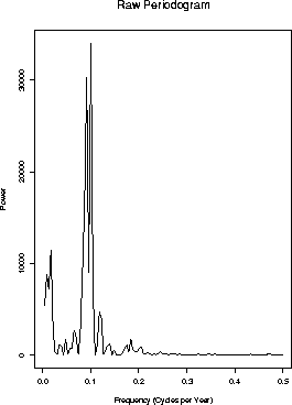
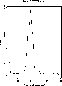
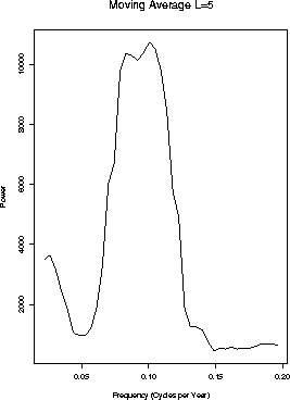
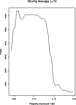
Here are several spectral estimates for the spectrum of the sunspots series:

• The raw periodogram. Are there two peaks near a period of 10 years? Is there a peak near 40 years?
  

• Running means with L=1.
  

• Running means L=5.
  

• Running means L=10.
  

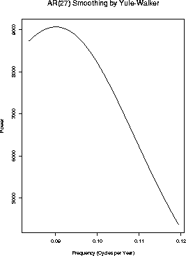
• Prewhitening by the AR(27) model selected by the use of AIC:
  

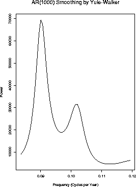
• Prewhitening by a high order AR(1000).