Postscript version of these notes

STAT 804

Lecture 20 Notes

Properties of Fourier Series

The Fourier series for a function f truncated to order K, namely

$$a_0 + \sum_{k=1}^K a_k \cos(2\pi k t) + \sum_{k=1}^K b_k \sin(2\pi k t) ,$$

where the coefficients are given by the Fourier integrals gives the best possible approximation to f as a linear combination of these sines and cosines in the following sense. Suppose we try to choose c_k and d_k to minimize

$$\int_0^1 \left[f(t)-f_K(t)\right]^2 \, dt$$

where

$$f_K(t) = c_0 + \sum_{k=1}^K c_k \cos(2\pi k t) + \sum_{k=1}^K d_k \sin(2\pi k t)$$

Squaring out the integrand and integrating term by term we get, remembering that the sines and cosines are orthogonal,

$$\begin{eqnarray*}\int_0^1 \left[f(t)-f_K(t)\right]^2 \, dt & = & \int_0^1 f^2(t)... ... f(t) \left[c_k\cos(2\pi k t) + d_k \sin(2\pi k t) \right] \, dt \end{eqnarray*}$$

Taking a derivative with respect to, say, c_j gives $c_j- int_0^1 f(t) \cos(2\pi j t) \, dt$which is 0 when c_j is the Fourier coefficient.

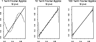
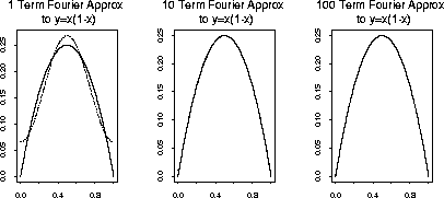
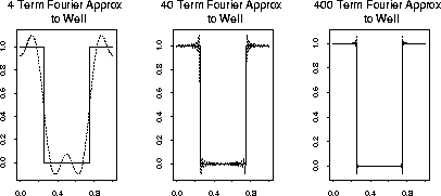
This result says that a Fourier series is the best possible approximation to a function f by a trigonometric polynomial of this type. However, the conclusion depends quite heavily on how we measure the quality of approximation. Below are Fourier approximations to each of 3 functions on [0,1]: the line y=x, the quadratic y=x(1-x) and the square well y=1(x<0.25)+1(y>0.75). For each plot the pictures get better as K improves. However the well shaped plot shows effects of Gibb's phenomenon: near the discontinuity in f there is an overshoot which is very narrow and spiky. The overshoot is of a size which does not depend on the order of approximation.

A similar discontinuity is implicit in the function y=x since the Fourier approximations are periodic with period 1. This means that the approximations are equal at 0 and at 1 while y=x is not. The quadratic function does have f(0)=f(1) and the Fourier approximation is much better.

My S-plus plotting code:

lin <-  function(k)
{
        x <- seq(0, 1, length = 5000)
        kv <- 1:k
        sv <- sin(2 * pi * outer(x, kv))
        y <-  - sv %*% (1/(pi * kv)) + 0.5
        plot(x, x, xlab = "", ylab = "", main = paste(as.character(k), 
                "Term Fourier Approximation to y=x"), type = "l")
        lines(x, y, lty = 2)
}

shows the use of the outer function and the paste function as well as how to avoid loops using matrix arithmetic.