next up previous
Postscript version of these notes

STAT 804

Lecture 17 Notes

Forecasting: an introduction

Given data $X_0,\ldots,X_{T-1}$ our goal will be to guess, or forecast, XT or more generally XT+r. There are a variety of ad hoc methods as well as a variety of statistically derived methods. I illustrate the ad hoc methods with the exponentially weighted moving average (EWMA). In this case we simply take

\begin{displaymath}{\hat X}_T = (X_{T-1} + a X_{T-2} + a^2 X_{T-3} +\cdots +a^{T-1}X_0)/c(a,T)
\end{displaymath}

where c(a,T) makes it a weighted average: c(a,T) =(1-aT)/(1-a). If we take a near to 1 we are almost using the sample mean while if we take a near 0 we are virtually using XT-1. You are supposed to choose a to trade off the desire to use lots of data against the possibility that the structure of the series has changed over time.

Statistically based methods concentrate on some measure of the size of $X_T-{\hat X}_T$; the mean squared prediction error ${\rm E}([X_T-{\hat X}_T]^2)$ is the most common.

In general ${\hat X}_T$ must be some function $f(X_0,\ldots,X_{t-1})$. The mean squared prediction error can be seen by conditioning on the data to be minimized by

\begin{displaymath}{\hat X}_T = {\rm E}(X_T\vert X_0,\ldots,X_{T-1})
\end{displaymath}

For most distributions of the X's this would be hard to compute but for Gaussian processes the solution is the usual linear regression of XT on the data, namely

\begin{displaymath}{\hat X}_T =\mu_T + a_1 (X_{T-1}-\mu_{T-1}) + \cdots a_T( X_0-\mu_{0})
\end{displaymath}

where the coefficient vector a is given by

\begin{displaymath}a= {\rm Cov}(X_T,( X_{T-1},\dots,X_0)^T) {\rm Var}(
X_{T-1},\dots,X_0)^{-1}
\end{displaymath}

When T is large the computation of these forecasts is difficult in general. There are some shortcuts, however.

Forecasting AR(p) processes

When the process is an AR the computation of the conditional expectation is easier:
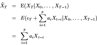
\begin{eqnarray*}{\hat X}_T & = & {\rm E}(X_T\vert X_0,\ldots,X_{T-1})
\\
& = ...
...-i} \vert X_0,\ldots,X_{T-1}) \\
& = & \sum_{i=1}^p a_iX_{t-i}
\end{eqnarray*}


For r>0 we have the recursion

\begin{eqnarray*}{\rm E}(X_{T+r}\vert X_0,\ldots,X_{T-1}) & = & E(\epsilon_{T+r}...
...X_0,\ldots,X_{T-1}) \\
& = & \sum_{i=1}^p a_i {\hat X}_{T+r-i}
\end{eqnarray*}


Notice the the forecast into the future uses current values where these are available and forecasts already calculated for the other X's.

Forecasting ARMA(p,q) processes

An ARMA(p,q) can be inverted to be an infinite order AR process. We could then use the method just given for the AR except that now the formula actually mentions values of Xtfor t < 0. In practice we simply truncate the series and ignore the missing terms in the forecast, assuming that the coefficients of these omitted terms are very small. Remember each term is built up out of a geometric series for $(I-\alpha B)^{-1}$ with $\vert\alpha\vert < 1$.

A more direct method goes like this:

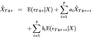
\begin{eqnarray*}{\hat X}_{T+r}& =& {\rm E}(\epsilon_{T+r}\vert X) + \sum_{i=1}^...
...-i} \\
& & + \sum_{i=1}^q b_i {\rm E}(\epsilon_{T+r-i}\vert X)
\end{eqnarray*}


where now the conditioning ``|X'' means given the observed data.

Whenever the time index on an epsilon is T or more the conditional expectations are 0. For T+r-i < T we need to guess the value of $\epsilon_{T+r-i}$. The same recurtion can be re-arranged to help compute ${\rm E}(\epsilon_t\vert X)$ for $0 \le t \le T-1$, at least approximately:

\begin{eqnarray*}{\rm E}(\epsilon_t\vert X) & = & X_t - \sum a_i X_{t-i} \\
& & + \sum b_i {\rm E}(\epsilon_{t-i}\vert X)
\end{eqnarray*}


This recursion works you backward but you have to get it started. Generally we start the recursion by putting

\begin{displaymath}{\hat\epsilon}_t = 0
\end{displaymath}

for negative t and then using the recursion. The coefficients bare such that the effect of getting these values of $\epsilon$ wrong is damped out at a geometric rate as we increase t so if we have enough data and the smallest root of the characteristic polynomial for the MA part is not too close to 1 then we will have accurate values for ${\hat\epsilon}_t$ for t near T.

As we discussed in the section on estimation these computed estimates of the epsilon's can be improved by backcasting the values of $\epsilon_t$ for negative t and then forecasting and backcasting, etc.

Forecasting ARIMA(p,d,q) series

If Z=(I-B)d X and X is ARIMA(p,d,q) then we: compute Z, forecast Z and reconstruct X by undoing the differencing. For d=1 for example we just have

\begin{displaymath}{\hat X}_{t} = {\hat Z}_t + {\hat X}_{t-1} \, .
\end{displaymath}

Forecast standard errors

You should remind yourself that the computations of conditional expectations we have just made used the fact that the a's and b's are constants - the true parameter values. In fact we then replace the parameter values with estimates. The quality of our forecasts will be summarized by the forecast standard error:

\begin{displaymath}\sqrt{{\rm E}[(X_t-{\hat X}_t)^2]} \, .
\end{displaymath}

We will compute this ignoring the estimation of the parameters and then discuss how much that might have cost us.

If ${\hat X}_t={\rm E}(X_t\vert X)$ then ${\rm E}({\hat X}_t) + {\rm E}(X_t)$so that our forecast standard error is just the variance of $X_t-{\hat X}_t$.

Consider first the case of an AR(1) and one step ahead forecasting:

\begin{displaymath}X_T-{\hat X}_T = \epsilon_T \, .
\end{displaymath}

The variance of this forecast is $\sigma_\epsilon^2$ so that the forecast standard error is just $\sigma_\epsilon$.

For forecasts further ahead in time we have

\begin{displaymath}{\hat X}_{T+r} = a {\hat X}_{T+r-1}
\end{displaymath}

and

\begin{displaymath}X_{T+r} = a X_{T+r-1} + \epsilon_{T+r}
\end{displaymath}

Subtracting we see that

\begin{displaymath}{\rm Var}(X_{T+r} -{\hat X}_{T+r}) = \sigma_\epsilon^2 + {\rm
Var}(X_{T+r-1}- {\hat X}_{T+r-1})
\end{displaymath}

so that we may calculate forecast standard errors recursively. As $r \to \infty$ we can check that the forecast variance converges to

\begin{displaymath}\sigma_\epsilon^2/(1-a^2)\end{displaymath}

which is simply the variance of individual Xs. When you forecast a stationary series far into the future the forecast error is just the standard deviation of the series.

Turn now to a general ARMA(p,q). Rewrite the process as the infinite order AR

\begin{displaymath}X_t = \sum_{s>0} c_s X_{t-s} + \epsilon_t
\end{displaymath}

to see that again, ignoring the truncation of the infinite sum in the forecast we have

\begin{displaymath}X_T -{\hat X}_T = \epsilon_T
\end{displaymath}

so that the one step ahead forecast standard error is again $\sigma_\epsilon$.

Parallel to the AR(1) argument we see that

\begin{displaymath}X_{T+r} - {\hat X}_{T+r} = \sum_{j=0}^{r-1} a_j ( X_{T+j} - {\hat X}_{T+j})
+ \epsilon_{T+r} \, .
\end{displaymath}

The errors on the right hand side are not independent of one another so that computation of the variance requires either computation of the covariances or recognition of the fact that the right hand side is a linear combination of $\epsilon_T, \ldots,\epsilon_{T+r}$.

A simpler approach is to write the process as an infinite order MA:

\begin{displaymath}X_t = \epsilon_t + \sum_{s>0} d_s\epsilon_{t-s}
\end{displaymath}

for suitable coefficients ds. Now if we treat conditioning on the data as being effectively equivalent to conditioning on all Xt for t < T we are effectively conditioning on $\epsilon_t$ for all t<T. This means that

\begin{eqnarray*}{\rm E}(X_{T+r}\vert X_{T-1}, X_{T-2},\ldots ) & = & {\rm E}(X_...
...ilon_{T-2}
, \ldots) \\
& = & \sum_{s >r} d_s \epsilon_{T+r-s}
\end{eqnarray*}


and the forecast error is just

\begin{displaymath}X_{T+r}-{\hat X}_{T+r} = \epsilon_t + \sum_{s=1}^r d_s\epsilon_{T+r-s}
\end{displaymath}

so that the forecast standard error is

\begin{displaymath}\sigma_\epsilon\sqrt{1 + \sum_{s=1}^r d_s^2} \, .
\end{displaymath}

Again as $r \to \infty$ this converges to $\sigma_X$.

Finally consider forecasting the ARIMA(p,d,q) process (I-B)d X= W where W is ARMA(p,q). The forecast errors in X can clearly be written as a linear combination of forecast errors for W permitting the forecast error in X to be written as a linear combination of the underlying errors $\epsilon_t$. As an example consider first the ARIMA(0,1,0) process $X_t=\epsilon_t+X_{t-1}$. The forecast of $\epsilon_{T+r}$ is just 0 and so the forcast of XT+r is just

\begin{displaymath}{\hat X}_{T+r} = {\hat X}_{T+r-1} = \cdots = X_{T-1}\, .
\end{displaymath}

The forecast error is

\begin{displaymath}\epsilon_{T+r} + \cdots + \epsilon_T
\end{displaymath}

whose standard deviation is $\sigma\sqrt{r+1}$. Notice that the forecast standard error grows to infinity as $r \to \infty$. For a general ARIMA(p,1,q) we have

\begin{displaymath}{\hat X}_{T+r} = {\hat X}_{T+r-1} +{\hat W}_{T+r}
\end{displaymath}

and

\begin{displaymath}X_{T+r} - {\hat X}_{T+r} = (W_{T+r} - {\hat W}_{T+r}) + \cdots + (W_T - {\hat W}_T)
\end{displaymath}

which can be combined with the expression above for the forecast error for an ARMA(p,q) to compute standard errors.

Software

The S-Plus function arima.forecast can do the forecasting.

Comments

I have ignored the effects of parameter estimation throughout. In ordinary least squares when we predict the Y corresponding to a new x we get a forecast standard error of

\begin{displaymath}\sqrt{Var(Y-x\hat\beta)} = \sqrt{Var(\epsilon + x(\beta-\hat\beta))}
\end{displaymath}

which is

\begin{displaymath}\sigma \sqrt{1+x(X^TX)^{-1} x^T} \, .
\end{displaymath}

The procedure used here corresponds to ignoring the term x(XTX)-1 xT which is the variance of the fitted value. Typically this value is rather smaller than the 1 to which it is added. In a 1 sample problem for instance it is simply 1/n. Generally the major component of forecast error is the standard error of the noise and the effect of parameter estimation is unimportant.


next up previous


Richard Lockhart
1999-10-13