


Postscript version of these notes
STAT 804
Lecture 11
Likelihood Theory
First we review likelihood theory for conditional and full
maiximum likelihood estimation.
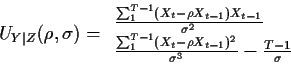
Suppose the data is X=(Y,Z) and write the density of X
as
Differentiate the identity
with respect to  (the jth component of
  )
and pull the derivative under the integral sign to get
)
and pull the derivative under the integral sign to get
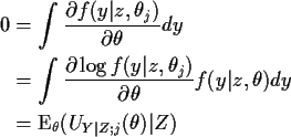
where
 is the jth component of
 ,
the derivative of the log conditional
likelihood; UY|Z is called a conditional score. Since
,
the derivative of the log conditional
likelihood; UY|Z is called a conditional score. Since
we may take expected values to see
that
It is also true
that the other two scores
 and
and
 have mean 0 (when
is the
true value of ).
Differentiate the identity a further time with respect to
have mean 0 (when
is the
true value of ).
Differentiate the identity a further time with respect to  to get
We define the conditional Fisher information matrix
 to have jkth entry
and get
The corresponding identities based on fX and fZ are
and
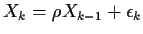
Now let's look at the model
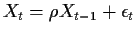 .
Putting
.
Putting
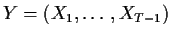 and Z=X0 we find
Differentiating again gives the matrix of second derivatives
Taking conditional expectations given X0 gives
To compute
![$W_k \equiv \text{E}[X_k^2\vert X_0]$](img24.gif) write
write
 and get
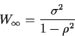
with W0=X02.
You can check carefully that in fact Wk converges to some  as
as
 .
This
satisfies
.
This
satisfies
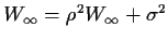 which gives
It follows that
Notice that although the conditional Fisher information
might have been expected to depend on X0 it does not, at least for
long series.
Richard Lockhart
1999-11-01

![\begin{displaymath}\text{E}
\left[- \frac{\partial^2 \ell}{\partial\theta_j\partial\theta_k}\vert Z\right]
\end{displaymath}](img15.gif)
![\begin{displaymath}\left[
\begin{array}{cc}
-\frac{\sum_1^{T-1}X_{t-1}^2}{\sigma...
...X_{t-1})^2}{\sigma^4} +\frac{T-1}{\sigma^2}
\end{array}\right]
\end{displaymath}](img22.gif)
![\begin{displaymath}I_{Y\vert Z}(\rho,\sigma) = \left[
\begin{array}{cc}
\frac{\s...
...igma^2}
&
0 \\ 0 &
\frac{2(T-1)}{\sigma^2}
\end{array}\right]
\end{displaymath}](img23.gif)
![\begin{displaymath}\frac{1}{T} I_{Y\vert Z}(\rho,\sigma) \to
\left[
\begin{arr...
...c{1}{1-\rho^2} & 0 \\ 0 & \frac{2}{\sigma^2}\end{array}\right]
\end{displaymath}](img31.gif)