Definition:
![]() iff
iff
Definition:
![]() iff
iff
![]() (a column vector for later use) with the
Zi independent and each
(a column vector for later use) with the
Zi independent and each
![]() .
.
In this case,

where the superscript t denotes matrix transpose.
Definition: ![]() has a multivariate normal distribution if it
has the same distribution as
has a multivariate normal distribution if it
has the same distribution as ![]() for some
for some
![]() ,
some
,
some
![]() matrix of constants A and
matrix of constants A and
![]() .
.
Lemma: The matrix A can be taken to be square with no loss of generality.
Proof: The simplest proof involves multivariate characteristic
functions:

If the matrix A is singular then X will not have a density. If A is
invertible then we can derive the multivariate normal density
by the change of variables formula:
Properties of the MVN distribution
![\begin{displaymath}X = \left[\begin{array}{c} X_1\\ X_2\end{array} \right]
\end{displaymath}](img23.gif)
![\begin{displaymath}\mu = \left[\begin{array}{c} \mu_1\\ \mu_2\end{array} \right]
\end{displaymath}](img24.gif)
![\begin{displaymath}\Sigma = \left[\begin{array}{cc} \Sigma_{11} & \Sigma_{12}
\\
\Sigma_{21} & \Sigma_{22} \end{array} \right]
\end{displaymath}](img25.gif)
If X is an AR(p) process then

![\begin{displaymath}\left[\begin{array}{cc}C(0) & C(q) \\ C(q) & C(0) \end{array}\right]
\end{displaymath}](img36.gif)
![\begin{displaymath}\left[\begin{array}{ccc}
C(1) & \cdots & C(p)
\\
C(q-1)& \cdots & C(q-p)
\end{array}\right]
\end{displaymath}](img40.gif)
To use this idea we define the partial autocorrelation function
to be
Qualitative idea: A plot of the sample partial
autocorrelation function (derived by replacing CX by ![]() in the definition of PACF) is examined. For an AR(p) process
this sample plot ought to drop suddenly to 0 for h>p.
in the definition of PACF) is examined. For an AR(p) process
this sample plot ought to drop suddenly to 0 for h>p.
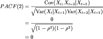
Now I calculate PACF(2) for a mean 0 AR(1) process. We have
![]() .
Let
.
Let
![\begin{displaymath}\left[\begin{array}{c}Y \\ Z\end{array}\right]
=
\left[\begin{array}{c} X_t \\ X_{t-2} \\ X_{t-1}\end{array}\right]
\end{displaymath}](img45.gif)
![\begin{displaymath}\Sigma = C_X(0)\left[\begin{array}{ccc}
1 & \rho^2 & \rho
\\
\rho^2 & 1 & \rho
\\
\rho & \rho & 1
\end{array}\right]
\end{displaymath}](img47.gif)
![\begin{displaymath}\Sigma_{11} = \Sigma = C_X(0)\left[\begin{array}{cc}
1 & \rho^2 \\ \rho^2 & 1\end{array}\right]
\end{displaymath}](img48.gif)
![\begin{displaymath}\Sigma_{12} = C_X(0)\left[\begin{array}{c}\rho\\ \rho \end{array} \right]
\end{displaymath}](img49.gif)
![\begin{align*}\text{Cov}(X_t,X_{t-2} \vert X_{t-1}) & = \Sigma_{11} - \Sigma_{12...
...t[\begin{array}{cc}
1-\rho^2 & 0 \\ 0 & 1-\rho^2 \end{array}\right]
\end{align*}](img51.gif)
Consider the problem of prediction Xt knowing
![]() .
In this course we choose a predictor
.
In this course we choose a predictor
![]() to minimize the mean squared prediction error:
to minimize the mean squared prediction error:
![\begin{displaymath}\text{E}(X_t\vert X_{t-1},\ldots,X_{t-K}) = \mu+A\left[\begin...
...}{c}
X_{t-1} - \mu \\ \vdots \\ X_{t-k}-\mu \end{array}\right]
\end{displaymath}](img57.gif)

![\begin{align*}\text{E}[(Y_t-\sum\alpha_i Y_{t-i})^2] & =
\text{E}(Y_t^2) - 2 \su...
...\
& = C(0) -2\sum\alpha_i C(i) + \sum_{ij} \alpha_i\alpha_j C(i-j)
\end{align*}](img63.gif)


Remark: This makes it look as if you would compute the
first 40 values of the PACF by solving 40 different problems and picking out the
last ![]() in each one but in fact there is an explicit recursive
algorithm to compute these things.
in each one but in fact there is an explicit recursive
algorithm to compute these things.
To estimate the PACF you can either estimate the ACF and do the arithmetic above with estimates instead of theoretical values or minimize a sample version of the mean squared prediction error:
The Mean Squared Prediction Error is
![\begin{displaymath}\text{E}\left\{[ (X_t - \mu - \sum_{j-1}^k \alpha_k (X_{t-k} - \mu)]^2\right\}
\end{displaymath}](img69.gif)
![\begin{displaymath}\sum_{t=k}^{T-1}\left \{[ (X_t -\bar{X}-\sum_{j-1}^k \alpha_k (X_{t-k} - \mu)]^2\right\}/T
\end{displaymath}](img71.gif)
![\begin{displaymath}Y = \left[\begin{array}{c} X_k-\bar{X} \\ \vdots \\ X_{T-1} - \bar{X}
\end{array}\right]
\end{displaymath}](img72.gif)
![\begin{displaymath}Z = \left[\begin{array}{ccc}
X_{t-1} - \bar{X} & \cdots & X_0...
...2} - \bar{X} & \cdots & X_{T-k-1} - \bar{X}
\end{array}\right]
\end{displaymath}](img73.gif)
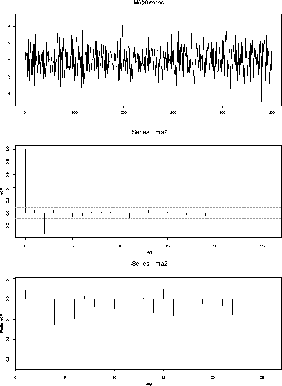
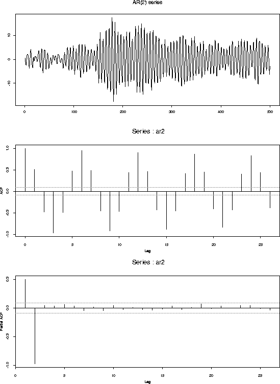
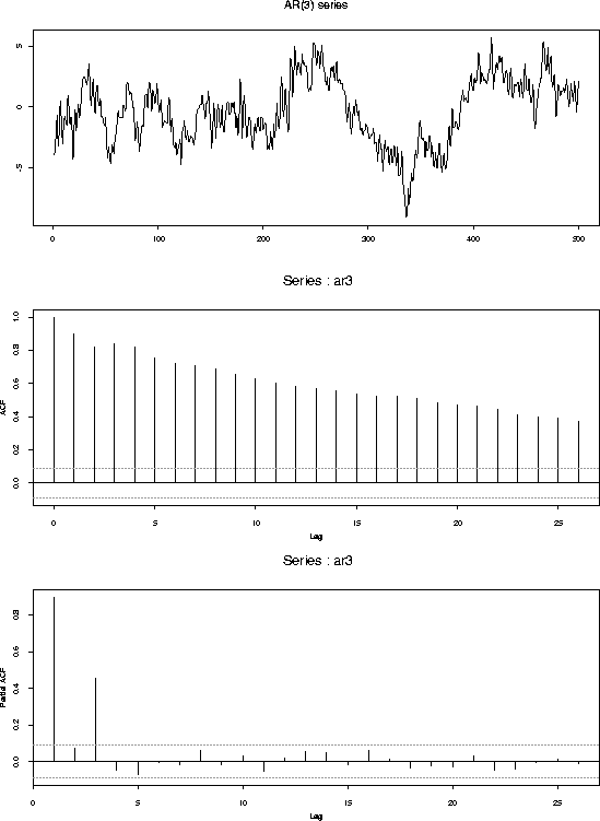
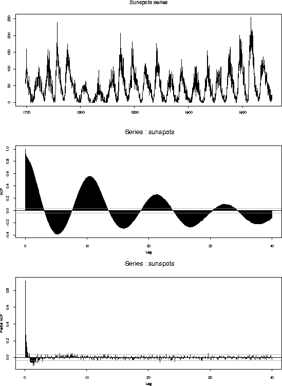
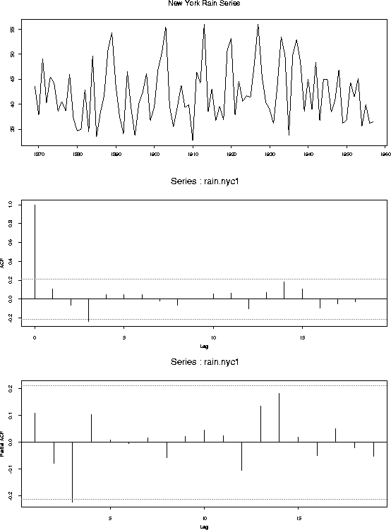
What follows are plots of 5 series, their fitted ACFs and their fitted PACFs. The series are:
Here is the SPlus code I used to make the following plots. You should note the use of the function acf which calculates and plots ACF and PACF.
#
# Comments begin with #
#
# Begin by generating the series.  The AR series generated are NOT
# stationary.  But I generate 10000 values from the recurrence relation
# and use the last 500. Asymptotic stationarity should guarantee that
# these last 500 are pretty stationary.
#
n<- 10000
ep <- rnorm(n)
ma2 <- ep[3:502]+0.8*ep[2:501]-0.9*ep[1:500]
ar2 <- rep(0,n)
ar2[1:2] <- ep[1:2]
for(i in 3:n) {ar2[i] <- ep[i]
              + ar2[i-1] -0.99*ar2[i-2]}
ar2 <- ar2[(n-499):n]
ar2 <- ts(ar2)
ar3 <- rep(0,n)
ar3[1:3] <- ep[1:3]
for(i in 4:n) {ar3[i] <- ep[i] + 0.8*ar3[i-1]
           -ar3[i-2]/3 +(0.8/1.712)*ar3[i-3]}
ar3 <- ar3[(n-499):n]
ar3 <- ts(ar3)
#
# The next line turns on a graphics device -- in this case the
# graph will be made in postscript in a file called ma2.ps. It
# will come out in portrait, not landscape, format.
#
postscript(file="ma2.ps",horizontal=F)
#
# The next line says to put 3 pictures
# in a single column on the plot
#
par(mfcol=c(3,1))
tsplot(ma2,main="MA(2) series")
acf(ma2)
acf(ma2,type="partial")
#
# When you finish a picture you turn
# off the graphics device
# with the next line.
#
dev.off()
#
#
#
postscript(file="ar2.ps",horizontal=F)
par(mfcol=c(3,1))
tsplot(ar2,main="AR(2) series")
acf(ar2)
acf(ar2,type="partial")
dev.off()
#
#
postscript(file="ar3.ps",horizontal=F)
par(mfcol=c(3,1))
tsplot(ar3,main="AR(3) series")
acf(ar3)
acf(ar3,type="partial")
dev.off()
#
#
postscript(file="sunspots.ps",horizontal=F)
par(mfcol=c(3,1))
tsplot(sunspots,main="Sunspots series")
acf(sunspots,lag.max=480)
acf(sunspots,lag.max=480,type="partial")
dev.off()
#
#
postscript(file="rain.nyc1.ps",horizontal=F)
par(mfcol=c(3,1))
tsplot(rain.nyc1,main="New York Rain Series")
acf(rain.nyc1)
acf(rain.nyc1,type="partial")
dev.off()
Sunspot data
New York City Rainfall
You should notice: