Postscript version of these notes

STAT 804: Notes on Lecture 4

More than 1 process

Definition: Two processes X and Y are jointly (strictly) stationary if

$${\cal L}(X_t,\ldots,X_{t+h},Y_t,\ldots,Y_{t+h}) = {\cal L}(X_0,\ldots,X_{h},Y_0,\ldots,Y_{h})$$

for all t and h. They are jointly second order stationary if each is second order stationary and also

$$C_{XY}(h) \equiv {\rm Cov}(X_t,Y_{t+h})={\rm Cov}(X_0,Y_{h})$$

for all t and h. Notice that negative values of h give, in general, different covariances than positive values of h.

Definition: If X is stationary then we call $C_X(h) = {\rm Cov}(X_0,X_h)$the autocovariance function of X.

Definition: If X and Y are jointly stationary then we call $C_{XY}(h) = {\rm Cov}(X_0,Y_h)$ the cross-covariance function.

Notice that C_X(-h) = C_X(h) and C_XY(h) = C_YX(-h) for all h and similarly for correlation

Definition: The autocorrelation function of X is

$$\rho_X(h) = C_X(h)/C_X(0) \equiv {\rm Corr}(X_0,X_h) \, .$$

the cross-correlation function of X and Y is

$$\rho_{XY}(h) = {\rm Corr}(X_0,Y_h)=C_{XY}(h)/\sqrt{C_X(0)C_Y(0)} \, .$$

Fact: If X and Y are jointly stationary then aX+bY is stationary for any constants a and b.

Model Identification

The goal of this section is to develop tools to permit us to choose a model for a given series X. We will be attempting to fit an ARMA(p,q) and our first step is to learn how to choose p and q. We will try to get small values of these orders and our efforts are focused on the cases with either p or q equal to 0. We use the autocorrelation or autocovariance function to do model identification.

Some Theoretical Autocovariances

1.

Moving Averages. Since addition of a constant never affects a covariance we take the mean equal to 0 and look at

$$X_t = \epsilon_t - \sum_1^p b_j\epsilon_{t-j}$$

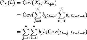
Using b₀=1 we find
$$\begin{align*}C_X(h) & = {\rm Cov}(X_t,X_{t+h}) \\ & = {\rm Cov}(\sum_{j=0}^p b... ...}^p \sum_{k=0}^p b_j b_k {\rm Cov}(\epsilon_{t-j},\epsilon_{t+h-k}) \end{align*}$$
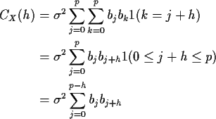
Each covariance is 0 unless t-j = t+h-k or k=j+h. This gives
$$\begin{align*}C_X(h) & =\sigma^2 \sum_{j=0}^p \sum_{k=0}^p b_j b_k 1(k=j+h) \\ ... ...j+h} 1(0 \le j+h \le p) \\ & = \sigma^2\sum_{j=0}^{p-h}b_j b_{j+h} \end{align*}$$

Notice that if h>p (or h < -p) then we get C_X(h) =0.

Jargon: We call h the lag and say that for an MA(p) process the autocovariance function is 0 at lags larger than p.

To identify an MA(p) look at a graph of an estimate $\hat{C}(h)$ and look for a lag where it suddenly decreases to (nearly) 0.

2.

Autoregressive Processes. Again we take $\mu=0$. Consider first p=1 so that $X_t = \rho X_{t-1} + \epsilon_t$. Then
$$\begin{align*}C_X(h) & = {\rm Cov}(X_t,X_{t+h}) \\ & ={\rm Cov}(X_t,\rho X_{t+h... ... & =\rho {\rm Cov}(X_t, X_{t+h-1}) + {\rm Cov}(X_t, \epsilon_{t+h}) \end{align*}$$

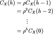
For h>0 the term ${\rm Cov}(X_t, \epsilon_{t+h})=0$. This gives
$$\begin{align*}C_X(h) & = \rho C_X(h-1) \\ & = \rho^2 C_X(h-2) \\ & \qquad \vdots \\ & = \rho^h C_X(0) \end{align*}$$
This gives

$$\rho_X(h) = \rho_X(1)^h = \rho^h$$

You should also recall that $C_X(0) = \sigma^2/(1-\rho^2)$.

Notice that R_X(h) decreases geometrically to 0 but is never actually 0.

Remark: If $\rho$ is small so that $\rho^2$ is very small then an AR(1) process is approximately the same as an MA(1) process: we nearly have $X_t = \epsilon_t + \rho \epsilon_{t-1}$.