Postscript version of this assignment

STAT 804: 99-3

Assignment 1

1.

Let $\epsilon_t$ be a Gaussian white noise process. Define

$$X_t=\epsilon_{t-2}+4\epsilon_{t-1}+6\epsilon_t +4\epsilon_{t+1}+\epsilon_{t+2} .$$

Compute and plot the autocovariance function of X.

2.

Suppose that X_t is strictly stationary.

(a)

If g is some function from R^p+1 to R show that

$$Y_t=g(X_t,X_{t-1},\ldots,X_{t-p})$$

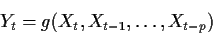
is strictly stationary.

(b)

What property must g have to guarantee the analogous result with strictly stationary replaced by $2^{\rm nd}$ order stationary? [Note: I expect a sufficient condition on g; you need not try to prove the condition is necessary.]

3.

Suppose that $\epsilon_t$ are iid and have mean 0 with finite variance. Verify that $X_t=\epsilon_t\epsilon_{t-1}$ is stationary and that it is wide sense white noise.

4.

Suppose X_t is a stationary Gaussian series with mean $\mu_X$and autocovariance R_X(k), $k=0, \pm 1, \ldots$. Show that $Y_t=\exp(X_t)$ is stationary and find its mean and autocovariance.

5.

Suppose that

$$X_t=a_1X_{t-1}+a_2X_{t-2}+\epsilon_t$$

where $\epsilon_t$ is an iid mean 0 sequence with variance $\sigma_\epsilon^2$. Compute the autocovariance function and plot the results for $\rho_1=0.2$ and $\rho_2=0.1$. (NOTE: I mean $\rho_i$ and NOT a_i here.) I have shown in class that the roots of a certain polynomial must have modulus more than 1 for there to be a stationary solution X for this difference equation. Translate the conditions on the roots $1/\alpha_1, 1/\alpha_2$ to get conditions on the coefficients a₁,a₂ and plot in the a₁,a₂ plane the region for which this process can be rewritten as a causal filter applied to the noise process $\epsilon_t$.

6.

Suppose that $\epsilon_t$ is an iid mean 0 variance $\sigma_\epsilon^2$sequence and that $a_t; t = 0, \pm 1, \pm2 ,\ldots$ are constants. Define

$$X_t = \sum a_s \epsilon_{t-s}$$

(a)

Derive the autocovariance of the process X.

(b)

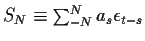
Show that $\sum a_s^2 < \infty$ implies

$$\lim_{N\to\infty} E[(X_t - \sum_{-N}^N a_s \epsilon_{t-s})^2] = 0$$

This condition shows that the infinite sum defining X converges ``in the sense of mean square''. It is possible to prove that this means that X can be defined properly. [Note: I don't expect much rigour in this calculation. Mathematically, you can't just define X_t as this question supposes since the sum is infinite. A rigourous treatment asks you to prove that the condition $\sum a_s^2 < \infty$ implies that the sequence $S_N \equiv \sum_{-N}^N a_s \epsilon_{t-s}$ is a Cauchy sequence in L². Then you have to know that this implies the existence of a limit in L² (technically, the point is that L² is a Banach space). Then you have to prove that the calculation you made in the first part of the question is mathematically justified.]

7.

Given a stationary mean 0 series X_t with autocorrelation $\rho_k$, $k=0, \pm 1, \ldots$and a fixed lag D find the value of A which minimizes the mean squared error

E[(X_t+d-AX_t)²]

and for the minimizing A evaluate the mean squared error in terms of the autocorrelation and the variance of X_t.

8.

The semivariogram of a stationary process X is

$$\gamma_X(m) = \frac{1}{2} E[(X_{t+m}-X_t)^2] \, .$$

(Without the 1/2 it's called the variogram.) Evaluate $\gamma$ in terms of the autocovariance of X.

DUE: Monday, 27 September.