Postscript version of this file

STAT 801 Lecture 7

Reading for Today's Lecture:

Goals of Today's Lecture:

• Examples of Fourier Inversion

• The local central limit theorem

• Convergence in distribution

Today's notes

Last time derived the Fourier inversion formula

$$f_X(x) = \frac{1}{2\pi} \int_{-\infty}^\infty \phi_X(u) e^{-iux} du$$

and the moment generating function inversion formula

$$2\pi i f(x) = \int_{-i\infty}^{i\infty} M(z) e^{-zx} dz$$

(where the limits of integration indicate a contour integral which runs up the imaginary axis.) The methods of complex variables permit this path to be replaced by any contour running up a line like Re(z)=c. (Re(Z) denotes the real part of z, that is, x when z=x+iy with x and y real.) The value of c has to be one for which $M(c) < \infty$. Rewrite the inversion formula using the cumulant generating function $K(t) = \log(M(t))$ to get

$$2\pi i f(x) = \int_{c-i\infty}^{c+i\infty} \exp(K(z)-zx) dz \, .$$

Along the contour in question we have z=c+iy so we can think of the integral as being

$$i\int_{-\infty}^\infty \exp(K(c+iy)-(c+iy)x) dy$$

Now do a Taylor expansion of the exponent:
$$\begin{multline*}K(c+iy)-(c+iy)x = \\ K(c)-cx +iy(K^\prime(c)-x)\\ -y^2 K^{\prime\prime}(c)/2+\cdots \end{multline*}$$
Ignore the higher order terms and select a c so that the first derivative

$$K^\prime(c)-x$$

vanishes. Such a c is a saddlepoint. We get the formula
$$\begin{multline*}2\pi f(x) \approx \exp(K(c)-cx)\\ \times \int_{-\infty}^\infty \exp(-y^2 K^{\prime\prime}(c)/2) dy \end{multline*}$$
The integral is just a normal density calculation and gives $\sqrt{2\pi/K^{\prime\prime}(c)}$. The saddlepoint approximation is

$$f(x)=\frac{\exp(K(c)-cx)}{\sqrt{2\pi K^{\prime\prime}(c)}}$$

Essentially the same idea lies at the heart of the proof of Sterling's approximation to the factorial function:

$$n! = \int_0^\infty \exp(n\log(x) -x) dx$$

The exponent is maximized when x=n. For n large we approximate $f(x) = n\log(x) -x$ by

$$f(x) \approx f(x_0) + (x-x_0) f^\prime(x_0) + (x-x_0)^2 f^{\prime\prime}(x_0)/2$$

and choose x₀ = n to make $f^\prime(x_0) = 0$. Then

$$n! \approx \int_0^\infty \exp[n\log(n) - n - (x-n)^2/(2n)] dx$$

Substitute $y = (x-n)/\sqrt{n}$ to get the approximation

$$n! \approx n^{1/2}n^n e^{-n} \int_{-\infty}^\infty e^{-y^2/2} dy$$

or

$$n! \approx \sqrt{2\pi} n^{n+1/2}e^{-n}$$

This tactic is called Laplace's method. Note that I am being very sloppy about the limits of integration; to do the thing properly you have to prove that the integral over x not near n is negligible.

Applications of Inversion

1): Numerical calculations

Example: Many statistics have a distribution which is approximately that of

$$T= \sum \lambda_j Z_j^2$$

where the Z_j are iid N(0,1). In this case
$$\begin{align*}E(e^{itT}) & = \prod E(e^{it\lambda_j Z_j^2}) \\ & = \prod (1-2it\lambda_j)^{-1/2} \, . \end{align*}$$
Imhof (Biometrika, 1961) gives a simplification of the Fourier inversion formula for

F_T(x) - F_T(0)

which can be evaluated numerically.

Here is how it works:
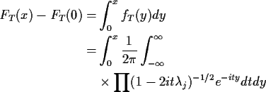
$$\begin{align*}F_T(x) - F_T(0) = & \int_0^x f_T(y) dy \\ = & \int_0^x \frac{1}{2... ...y}^\infty \\ & \times\prod (1-2it\lambda_j)^{-1/2} e^{-ity} dt dy \end{align*}$$
Multiply

$$\phi(t) = \left[\frac{1}{\prod(1-2it\lambda_j)}\right]^{1/2}$$

top and bottom by the complex conjugate of the denominator:

$$\phi(t) = \left[\frac{\prod(1+2it\lambda_j)}{\prod(1+4t^2\lambda_j^2)}\right]^{1/2}$$

The complex number $1+2it\lambda_j$ is $r_j e^{i\theta_j}$where $r_j = \sqrt{1+4t^4\lambda_j^2}$ and $\tan(\theta_j) = 2t\lambda_j$This allows us to rewrite

$$\phi(t) = \left[\frac{\prod r_j e^{i\sum\theta_j}}{\prod r_j^2}\right]^{1/2}$$

or

$$\phi(t) = \frac{ e^{i\sum\tan^{-1}(2t\lambda_j)/2} }{ \prod(1+4t^2\lambda_j^2)^{1/4} }$$

Assemble this to give

$$F_T(x) - F_T(0) = \frac{1}{2\pi} \int_{-\infty}^\infty \frac{ e^{i\theta(t)} }{ \rho(t) } \int_0^x e^{-iyt}dy dt$$

where

$$\theta(t) = \sum \tan^{-1}(2t\lambda_j) /2$$

and $\rho(t) = \prod(1+4t^2\lambda_j^2)^{1/4}$. But

$$\int_0^x e^{-iyt}dy = \frac{e^{-ixt}-1}{-it}$$

We can now collect up the real part of the resulting integral to derive the formula given by Imhof. I don't produce the details here.

2): The central limit theorem (the version which is called ``local'') can be deduced from the Fourier inversion formula: if $X_1,\ldots,X_n$ are iid with mean 0 and variance 1 and $T=n^{1/2}\bar{X}$ then with $\phi$ denoting the characteristic function of a single X we have
$$\begin{align*}E(e^{itT}) = & E(e^{in^{-1/2} t\sum X_j}) \\ = & \left[\phi(n^{-... ...\ & \left.+ n^{-1}t^2\phi^{\prime\prime}(0)/2 + o(n^{-1})\right]^n \end{align*}$$
But now $\phi(0) = 1$ and

$$\phi^\prime(t) = \frac{d}{dt} E(e^{itX_1}) = iE(X_1e^{itX_1})$$

So $\phi^\prime(0) = E(X_1) =0$. Similarly

$$\phi^{\prime\prime}(t) = i^2 E(X_1^2e^{itX_1})$$

so that

$$\phi^{\prime\prime}(0) = -E(X_1^2) =-1$$

It now follows that
$$\begin{align*}E(e^{itT}) & \approx [1-t^2/(2n) + o(1/n)]^n \\ & \to e^{-t^2/2} \end{align*}$$
With care we can then apply the Fourier inversion formula and get
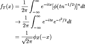
$$\begin{align*}f_T(x) & = \frac{1}{2\pi } \int_{-\infty}^\infty e^{-itx} [\phi(tn... ...infty e^{-itx} e^{-t^2/2} dt \\ &=\frac{1}{\sqrt{2\pi}} \phi_Z(-x) \end{align*}$$
where $\phi_Z$ is the characteristic function of a standard normal variable Z. Doing the integral we find

$$\phi_Z(x) = \phi_Z(-x) = e^{-x^2/2}$$

so that

$$f_T(x) \to \frac{1}{\sqrt{2\pi}} e^{-x^2/2}$$

which is a standard normal random variable.

This proof of the central limit theorem is not terribly general since it requires T to have a bounded continuous density. The usual central limit theorem is a statement about cdfs not densities and is

$$P(T \le t) \to P(Z \le t)$$

Convergence in Distribution

In undergraduate courses we often teach the central limit theorem as follows: if $X_1,\ldots,X_n$ are iid from a population with mean $\mu$ and standard deviation $\sigma$ then $n^{1/2}(\bar{X}-\mu)/\sigma$ has approximately a normal distribution. We also say that a Binomial(n,p) random variable has approximately a N(np,np(1-p)) distribution.

To make precise sense of these assertions we need to assign a meaning to statements like ``X and Y have approximately the same distribution''. The meaning we want to give is that X and Y have nearly the same cdf but even here we need some care. If n is a large number is the N(0,1/n) distribution close to the distribution of $X\equiv 0$? Is it close to the N(1/n,1/n) distribution? Is it close to the $N(1/\sqrt{n},1/n)$ distribution? If $X_n\equiv 2^{-n}$ is the distribution of X_n close to that of $X\equiv 0$?

The answer to these questions depends in part on how close close needs to be so it's a matter of definition. In practice the usual sort of approximation we want to make is to say that some random variable X, say, has nearly some continuous distribution, like N(0,1). In this case we must want to calculate probabilities like P(X>x) and know that this is nearly P(N(0,1) > x). The real difficulty arises in the case of discrete random variables; in this course we will not actually need to approximate a distribution by a discrete distribution.

When mathematicians say two things are close together they mean one of two things: either they can provide an upper bound on the distance between the two things or they are talking about taking a limit. In this course we do the latter.

Definition: A sequence of random variables X_n converges in distribution to a random variable X if

$$E(g(X_n)) \to E(g(X))$$

for every bounded continuous function g.

Theorem 1   The following are equivalent:

1.

X_n converges in distribution to X.

2.

$P(X_n \le x) \to P(X \le x)$ for each x such that P(X=x)=0

3.

The limit of the characteristic functions of X_n is the characteristic function of X:

$$E(e^{itX_n}) \to E(e^{itX})$$

for every real x.

These are all implied by

$$M_{X_n}(t) \to M_X(t) < \infty$$

for all $\vert t\vert \le \epsilon$ for some positive $\epsilon$.

Now let's go back to the questions I asked:

• $X_n\sim N(0,1/n)$ and X=0. Then
  
  $$P(X_n \le x) \to \left\{\begin{array}{ll} 1 & x>0 \\ 0 & x<0 \\ 1/2 & x=0 \end{array}\right.$$
  
  
  Now the limit is the cdf of X=0 except for x=0 and the cdf of X is not continuous at x=0 so yes, X_n converges to X in distribution.

• I asked if $X_n\sim N(1/n,1/n)$ had a distribution close to that of $Y_n \sim N(0,1/n)$. The definition I gave really requires me to answer by finding a limit X and proving that both X_n and Y_nconverge to X in distribution. Take X=0. Then
  
  $$E(e^{tX_n}) = e^{t/n+t^2/(2n)} \to 1 = E(e^{tX})$$
  
  
  and
  
  $$E(e^{tY_n}) = e^{t^2/(2n)} \to 1$$
  
  
  so that both X_n and Y_n have the same limit in distribution.

• Multiply both X_n and Y_n by n^1/2 and let $X \sim N(0,1)$. Then $\sqrt{n}X_n \sim N(n^{-1/2},1)$ and $\sqrt{n} Y_n \sim N(0,1)$. Use characteristic functions to prove that both $\sqrt{n}X_n$ and $\sqrt{n} Y_n$ converge to N(0,1) in distribution.

• If you now let $X_n \sim N(n^{-1/2},1/n)$ and $Y_n \sim N(0,1/n)$then again both X_n and Y_n converge to 0 in distribution.

• If you multiply X_n and Y_n in the previous point by n^1/2 then $n^{1/2}X_n \sim N(1,1)$ and $n^{1/2} Y_n \sim N(0,1)$ so that n^1/2X_nand n^1/2 Y_n are not close together in distribution.

• You can check that $2^{-n}\to 0$ in distribution.

Here is the message you are supposed to take away from this discussion. You do distributional approximations by showing that a sequence of random variables X_n converges to some X. The limit distribution should be non-trivial, like say N(0,1). We don't say X_n is approximately N(1/n,1/n) but that n^1/2 X_n converges to N(0,1) in distribution.