Brownian Motion
For fair random walk ![]() = number of heads minus number of
tails,
= number of heads minus number of
tails,
![]()
where the ![]() are independent and
are independent and
![]()
Notice:
![]()
Recall central limit theorem:
![]()
Now: rescale time axis so that n steps take 1 time unit
and vertical axis so step size is ![]() .
.
We now turn these pictures into a stochastic process:
For ![]() we define
we define
![]()
Notice:
![]()
and
![]()
As ![]() with t fixed we see
with t fixed we see ![]() . Moreover:
. Moreover:
![]()
converges to N(0,1) by the central limit theorem. Thus
![]()
Another observation:
![]() is independent of
is independent of ![]() because the
two rvs involve sums of different
because the
two rvs involve sums of different ![]() .
.
Conclusions.
As ![]() the processes
the processes ![]() converge to a process
X with the properties:
converge to a process
X with the properties:
![]()
then
![]()
are independent .
![]()
regardless of s.
Def'n: Any process satisfying 1-4 above is a Brownian motion.
Properties of Brownian motion

Notice the use of independent increments and of ![]() .
.

Suppose t< s. Then ![]() is a sum
of two independent normal variables. Do following calculation:
is a sum
of two independent normal variables. Do following calculation:
![]() , and
, and ![]() independent. Z=X+Y.
independent. Z=X+Y.
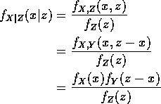
Compute conditional distribution of X given Z:

Now Z is ![]() where
where ![]() so
so

for suitable choices of a and b. To find them compare coefficients
of ![]() , x and 1.
, x and 1.
Coefficient of ![]() :
:
![]()
so ![]() .
.
Coefficient of x:
![]()
so that
![]()
Finally you should check that
![]()
to make sure the coefficients of 1 work out as well.
Conclusion: given Z=z the conditional distribution of X is
![]() with a and b as above.
with a and b as above.
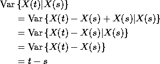
Application to Brownian motion:
![]()
and
![]()
SO:
![]()
and
![]()