Postscript version of these notes

STAT 350: Lecture 13

Reading: Chapter 9.

Sand and Fibre Analysis so far:

1.

F test of H_o: no quadratic terms accepted the null.

2.

F test of $\beta_1 = \beta_3 =0$ in the model

$$Y_i = \beta_0 + \beta_1 S_i + \beta_3 F_i + \epsilon_i$$

rejects.

Next

3.

t tests of $\beta_1 =0$ (t on 15 df)

$$\frac{\hat\beta_1}{s_{\hat\beta_1}} \equiv \frac{\hat\beta_1}{\hat\sigma_{\hat\beta_1}} = 3.75 \qquad P = 0.0019$$

Remark: This can be done in the quadratic model too.

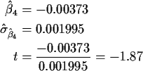
Conclusion: $\beta_1 \neq 0$; Sand has an impact on Y.

Similarly $\beta_3 \neq 0$.

4.

Is final model

$$Y_i = \hat\beta_0 + \hat\beta_1 S_i + \hat\beta_3 F_i +\hat\epsilon_i$$

adequate?

Assessing model fit

Informal methods:

1.

Plot residuals $\hat\epsilon_i$ against each x_i, i.e. against S_i and F_i.

2.

Plot residuals against other covariates, particularly those deleted from model.

3.

Plot residuals against $\hat\mu_i$ = fitted value.

Look for:

(a)

Curvature -- suggesting need of x² or non-linear model.

(b)

Heteroscedasticity.

(c)

Omitted variables.

4.

Plot order statistics of residuals against quantiles of N(0,1): a Q-Q plot.

$$\hat\epsilon_{(1)} < \hat\epsilon_{(2)} < \cdots < \hat\epsilon_{(n)}$$

are the $\hat\epsilon_1, \ldots,\hat\epsilon_n$ arranged in increasing order -- called ``order statistics''.

$$h_1 < \cdots < h_n$$

are ``Normal scores''. They are defined by the equation

$$P(N(0,1) \le h_i) = \frac{i}{n+1}$$

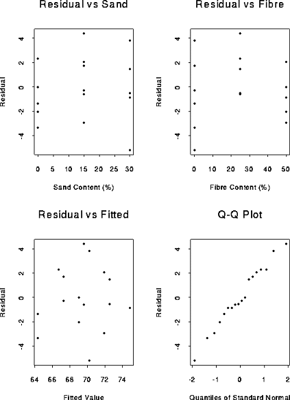
Here are some plots:

Conclusions from the plots.

• Q-Q plot is reasonably straight. So normality is OK and t and F tests should work well.

• The plot of residual versus fitted values is more or less OK.

  Warning: don't look too hard for patterns; you will find them where they aren't.

• The plot of residual versus Sand is ok.

• The plot of residual versus Fibre has mostly positive residuals for the middle values of Fibre suggesting a quadratic pattern. So, we compare
  
  $$Y = \beta_0 + \beta_1 S + \beta_3 F + \epsilon$$
  
  
  and
  
  $$Y = \beta_0 + \beta_1 S + \beta_3 F +\beta_4 F^2+ \epsilon$$
  
  
  We can use a t test on $\beta_4$ to test $H_o:\beta_4 = 0$ in the second of these models. We find
  $$\begin{align*}\hat\beta_4 & = -0.00373 \\ \hat\sigma_{\hat\beta_4} &= 0.001995 \\ t & = \frac{-0.00373}{0.001995} = -1.87 \end{align*}$$
  based on 18 degrees of freedom so we get the marginally not significant P value 0.08.

Conclusion: evidence of need for the F² term is weak. We might want more data if the ``optimal'' Fibre content is needed.

Notice as always: statistics does not eliminate uncertainty but rather quantifies it.

More formal model assessment tools

1.

Fit larger model: test for non-zero coefficients. We did this to compare linear to full quadratic model.

2.

Look for outlying residuals.

Standardized / studentized residuals

Recall that

$$\hat\epsilon \sim MVN(0,\sigma^2(I-H))$$

It follows that

$$\hat\epsilon_i \sim N(0,\sigma^2(1-h_{ii}))$$

where h_ii is the iith diagonal entry in H. Thus

$$\frac{\hat\epsilon_i}{\sigma\sqrt{1-h_{ii}}} \sim N(0,1)$$

This is not useful yet since $\sigma$ is unknown. However we can replace $\sigma$ with the obvious estimate and find that

$$\frac{\hat\epsilon_i}{\hat\sigma\sqrt{1-h_{ii}}} \sim N(0,1)$$

provided that n is large. This is called an internally studentized or standardized residual. The suggestion is to look for standard residuals larger than about 2.

Warning: the N((0,1) approximation requires normal errors.

Criticism of internally standardized residuals. If the model is bad particularly at point i then including point i pulls the fit towards Y_i, inflates $\hat\sigma$ and makes the badness hard to see.

Suggestion: for each point i delete point i, refit the model, predict Y_i (call the prediction $\hat{Y}_{i(i)}$ where the (i) in the subscript shows which point was deleted. We then get case deleted residuals

$$Y_i - \hat{Y}_{i(i)}$$

Standardized Residuals

For the insurance data we can look at the residuals after various model fits.

data insure;
  infile 'insure.dat' firstobs=2;
  input year cost;
  code = year - 1975.5 ;
proc glm  data=insure;
   model cost = code ;
   output out=insfit h=leverage p=fitted r=resid student=isr press=press rstudent=esr;
run ;
proc print data=insfit ;
run;
proc glm  data=insure;
   model cost = code code*code code*code*code ;
   output out=insfit3 h=leverage p=fitted r=resid student=isr press=press rstudent=esr;
run ;
proc print data=insfit3 ;
run;
proc glm  data=insure;
   model cost = code code*code code*code*code code*code*code*code code*code*code*code*code;
   output out=insfit5 h=leverage p=fitted r=resid student=isr press=press rstudent=esr;
run ;
proc print data=insfit5 ;
run;

The full output is here but I reproduce parts of it here.

For the linear fit:

   OBS YEAR  COST  CODE LEVERAGE  FITTED   RESID     ISR     PRESS     ESR

     1 1971  45.13 -4.5  0.34545 42.5196   2.6104  0.36998   3.9881  0.34909
     2 1972  51.71 -3.5  0.24848 48.8713   2.8387  0.37550   3.7773  0.35438
     3 1973  60.17 -2.5  0.17576 55.2229   4.9471  0.62485   6.0020  0.59930
     4 1974  64.83 -1.5  0.12727 61.5745   3.2555  0.39960   3.7302  0.37758
     5 1975  65.24 -0.5  0.10303 67.9262  -2.6862 -0.32524  -2.9947 -0.30626
     6 1976  65.17  0.5  0.10303 74.2778  -9.1078 -1.10275 -10.1540 -1.12017
     7 1977  67.65  1.5  0.12727 80.6295 -12.9795 -1.59320 -14.8723 -1.80365
     8 1978  79.80  2.5  0.17576 86.9811  -7.1811 -0.90702  -8.7124 -0.89574
     9 1979  96.13  3.5  0.24848 93.3327   2.7973  0.37001   3.7222  0.34912
    10 1980 115.19  4.5  0.34545 99.6844  15.5056  2.19772  23.6892  3.26579

In this case it is the pattern of the residuals, together with the big improvement in moving to a cubic model (as measured by the drop in ESS), which convinces us that the linear fit is bad. You will see that the leverages are not too large, that the internally studentized residuals are mostly acceptable though the 2.2 for 1980 is a bit big. However the externally standard residual for 1980 is really much too big.

Now for the cubic fit:

   OBS YEAR  COST  CODE LEVERAGE  FITTED   RESID     ISR     PRESS     ESR

     1 1971  45.13 -4.5  0.82378  43.972  1.15814  1.21745  6.57198  1.28077
     2 1972  51.71 -3.5  0.30163  54.404 -2.69386 -1.42251 -3.85737 -1.59512
     3 1973  60.17 -2.5  0.32611  60.029  0.14061  0.07559  0.20865  0.06903
     4 1974  64.83 -1.5  0.30746  62.651  2.17852  1.15521  3.14570  1.19591
     5 1975  65.24 -0.5  0.24103  64.073  1.16683  0.59104  1.53738  0.55597
     6 1976  65.17  0.5  0.24103  66.098 -0.92750 -0.46981 -1.22205 -0.43699
     7 1977  67.65  1.5  0.30746  70.528 -2.87752 -1.52587 -4.15503 -1.78061
     8 1978  79.80  2.5  0.32611  79.166  0.63372  0.34066  0.94039  0.31403
     9 1979  96.13  3.5  0.30163  93.817  2.31320  1.22150  3.31229  1.28644
    10 1980 115.19  4.5  0.82378 116.282 -1.09214 -1.14807 -6.19746 -1.18642

Now the fit is generally ok with all the standardized residuals being fine. Notice the large leverages for the end points, 1971 and 1980.

Finally the quintic:

   OBS YEAR  COST  CODE LEVERAGE  FITTED   RESID     ISR     PRESS     ESR

     1 1971  45.13 -4.5  0.98322  45.127  0.00312  0.03977  0.18583  0.03445
     2 1972  51.71 -3.5  0.72214  51.699  0.01090  0.03417  0.03924  0.02960
     3 1973  60.17 -2.5  0.42844  60.232 -0.06161 -0.13462 -0.10780 -0.11685
     4 1974  64.83 -1.5  0.46573  64.784  0.04641  0.10487  0.08686  0.09095
     5 1975  65.24 -0.5  0.40047  65.228  0.01181  0.02520  0.01970  0.02183
     6 1976  65.17  0.5  0.40047  64.925  0.24502  0.52270  0.40868  0.46897
     7 1977  67.65  1.5  0.46573  68.392 -0.74249 -1.67794 -1.38974 -2.67034
     8 1978  79.80  2.5  0.42844  78.981  0.81942  1.79036  1.43365  3.47878
     9 1979  96.13  3.5  0.72214  96.543 -0.41296 -1.29407 -1.48622 -1.46985
    10 1980 115.19  4.5  0.98322 115.110  0.08038  1.02486  4.78917  1.03356

Now notice that the leverages at the end are very high and that although the fit is good the residuals at 1977 and 1978 are definitely too big. Overall the cubic fit is to be preferred but does not provide reliable forecasts nor a meaningful physical description of the data. A good model would somehow involve economic theory and covariates, though there is really very little data to fit such models.

How to make high quality graphs in SAS

The graphs produced by proc plot is SAS are intended to be printed on the most old fashioned printers. Better graphs can be made using proc gplot. The following code:

  data plaster;
  infile 'plaster.dat';
  input sand fibre hardness strength;
  proc glm  data=plaster;
   model hardness = sand fibre ;
   output out=outdat p=fitted r=resid h=leverage 
     cookd=cookd dffits=dffits rstudent=rstudent;
  run;
  proc rank data=outdat normal=vw out=outdat1;
   var resid;
   ranks normscr;
  run;
  proc gplot data=outdat1;
   title3 'Residual Plots';
   plot resid*sand ;
   plot resid*fibre ;
   plot resid*fitted ;
   plot resid*normscr;
  run;

produces much higher quality graphs. First in proc glm we regress hardness on sand and fibre content. The output statement saves the residuals and fitted values, along with some regression diagnostics used in the next few lectures in a new data set called outdat. Then proc rank computes the normal scores which corresponding to the residuals and adds these normal scores to the data set making the new data set outdat1. Finally proc gplot graphs resid against sand, fibre, fitted value and the normal scores. The graphs which result are much easier to interpret.