Postscript version of these notes

STAT 350: Lecture 12

Reading: Chapter 7.

Extra Sum of Squares

Suppose we are fitting a model of the form

$$Y = [X_1 \vert X_2 ] \left[ \begin{array}{c} \beta_1 \\ \hline \beta_2 \end{array}\right] + \epsilon$$

We can test the hypothesis $H_o: \beta_2 = 0$ using the F test:

$$F = \frac{{\rm Extra SS} / {\rm dim}(\beta_2)}{{\rm ESS}_{\rm FULL}/ (n - p)} \sim F_{{\rm dim}(\beta_2),n-p}$$

where p is the total number of columns of the design matrix X=[X₁ | X₂ ] and
$$\begin{align*}{\rm Extra SS} & = \mbox{Error SS in } Y=X_1\beta_1 + \epsilon \\ & - \mbox{Error SS in } Y=X_1\beta_1+X_2 \beta_2 + \epsilon \end{align*}$$

ANOVA tables

The calculations for the test above are usually recorded in an ANalysis Of VAriance (ANOVA) table. Generally the design matrix will have a column of ones and we adjust the entries in the table for the grand mean $\bar{Y}$. In this case we have

$$X=[{\bf 1} \vert X_1 \vert X_2 ]$$

where X₁ has p₁ columns, X₂ has p₂ columns and there are a total of 1+p₁+p₂ parameters in the parameter vector

$$\beta = \left[ \begin{array}{c} \beta_0 \\ \hline \beta_1 \\ \hline \beta_2 \end{array}\right]$$

We use the notation p=p₁+p₂ but you must be careful: don't memorize formulas - learn to count columns. We decompose the data as

$$Y = {\bf 1} \bar{Y} + (\hat\mu_R - {\bf 1} \bar{Y}) + (\hat\mu_F -\hat\mu_R) + \hat\epsilon$$

The components are mutually orthogonal so that we get the sum of squares identity

$$\vert\vert Y-{\bf 1} \bar{Y}\vert\vert^2 = \vert\vert\hat\mu_... ...u_F-\hat\mu_R\vert\vert^2 + \vert\vert\hat\epsilon\vert\vert^2$$

which we normally put into an ANOVA table:

Source	Sum of Squares	Degrees of Freedom
X1	$\vert\vert\hat\mu_R - {\bf 1} \bar{Y}\vert\vert^2$	p1
X2|X1	$\vert\vert\hat\mu_F-\hat\mu_R\vert\vert^2$	p2
Error	$\vert\vert\hat\epsilon\vert\vert^2$	n-p-1
Total (Corrected)	$\sum(Y_i - \bar{Y})^2$	n-1

Typically we add a column of mean squares, always obtained by dividing the SS column by the degrees of freedom column, a column of F statistics, obtained by dividing the Mean Square by the MSE and a column of P values obtained from software which computes F distribution tail areas.

In this table the notation X₂|X₁ means X₂ adjusted for X₁ or X₂ after fitting X₁.

Analysis of SAND / FIBRE / HARDNESS of plaster example

We regress Y, the hardness of a plaster sample on S, S², F, F² and SF. There are 5 factors so there are 2⁵=32 possible submodels of the full model

$$Y_i = \beta_0 + \beta_1 S_i + \beta_2 S_i^2 + \beta_3 F_i + \beta_4 F_i^2 + \beta_5 S_i F_i + \epsilon_i$$

Many of these 32 models are not sensible, such as

$$Y_i = \beta_0 + \beta_4 F_i^2 + \epsilon_i$$

or

$$Y_i = \beta_0 + \beta_5 S_iF_i + \epsilon_i$$

The term $\beta_5 S_iF_i$ is an interaction of S and F. We analyze the data as follows:

Q: Are the effects of S and F additive?

A: Test $H_o: \beta_5 = 0$.

There are two methods to carry out such a test:

1.

A t test

2.

A F test.

Fact: the F test is equivalent to a two sided t test.

The t test uses

$$t= \frac{\hat\beta_5 - 0}{\hat\sigma_{\hat\beta_5}} = \frac{... ...eta_5}{\sqrt{{\rm MSE}}\sqrt{(X^TX)^{-1}_{66}}} \sim t_{1,n-6}$$

This is exactly the same as the Lecture 10 formula since

$$\beta_5 = \underbrace{[0,0,0,0,0,1]}_{x^T}\left[ \begin{array}{c} \beta_0 \\ \beta_1 \\ \vdots \\ \beta_5 \end{array}\right]$$

and x^T(X^TX)^-1 x is the lower right hand corner entry in (X^TX)^-1, that is, (X^TX)^-1₆₆.

The F test uses

$$F = \frac{({\rm ESS}_{\rm R} -{\rm ESS}_F) / 1}{{\rm ESS}_{\rm FULL}/ (n - 6)} \sim F_{1,n-6} \quad ( = t^2)$$

Proof by example:

The Data

• Y = hardness of plaster. n=18 batches.

• S = sand content. Values used 0%, 15% 30%.

• F = fibre content. Values used 0%, 25% 50%.

• Factorial design with 2 replicates.

Sand  Fibre  Hardness  Strength 
   0    0       61       34
   0    0       63       16
  15    0       67       36
  15    0       69       19
  30    0       65       28
     ...

``Full'' model

$$Y_i = \beta_0+\beta_1 S_i + \beta_2 S_i^2 + \beta_3 F_i + \beta_4 F_i^2 + \beta_5 S_i F_I + \epsilon_i$$

Fitted Models, ESS, df for error

Model for $\mu$	ESS	Error df
Full	81.264	12
$\beta_0+\beta_1 S_i + \beta_2 S_i^2 + \beta_3 F_i + \beta_4 F_i^2$	82.389	13
$\beta_0+\beta_1 S_i + \beta_2 S_i^2 + \beta_3 F_i$	104.167	14
$\beta_0+\beta_1 S_i + \beta_2 S_i^2$	169.500	15
$\beta_0+\beta_1 S_i$	174.194	16
$\beta_0+\beta_1 S_i + \beta_3 F_i + \beta_4 F_i^2$	87.083	14
$\beta_0+\beta_1 F_i + \beta_2 F_i^2$	189.167	15
$\beta_0+\beta_1 F_i$	210.944	16
$\beta_0+\beta_1 S_i + \beta_3 F_i$	108.861	15
$\beta_0$(empty model)	276.278	17

Hypothesis tests:

1.

Quadratic terms needed? $H_o: \beta_2=\beta_4=\beta_5=0$. Extra SS = 108.861-81.264. F=[ (108.861-81.264)/3]/[81.264/12]= 1.358. Degrees of freedom are 3,12 so P=0.30, not significant.

2.

Linear terms needed? There are several possible F-tests.

(a)

Compare full model to empty model.

F=(276.278-81.264)/5/(81.264/12) = 5.76

so P is about .006.

(b)

Assume full model is now additive, linear model

$$\beta_0+\beta_1 S_i + \beta_3 F_i .$$

Then

F=[(276.278-108.861)/2]/[108.861/15] = 11.53

and P is about 0.0009.

(c)

Use estimate of $\sigma^2$ from full model but get extra SS from last comparison: F=[(276.278-108.861)/2]/[81.264/12] = 12.36 for a P value of 0.001

Conclusions

• Both Sand and Fibre influence Hardness.

• Linear terms in S and F are adequate.

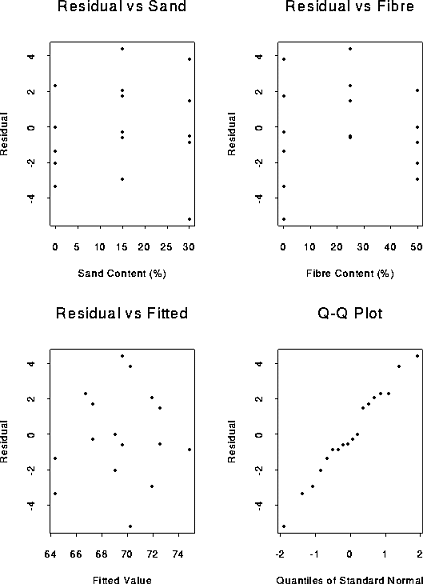
You should also examine residual plots. Here is a page of plots:

You will see that the plot of residual against fitted value suggests that we should consider adding a quadratic term in Fibre:

The model

$$Y_i = \beta_0+\beta_1 S_i + \beta_3 F_i + \beta_4 F_i^2 +\epsilon_i$$

has ESS=87.083 on 14 degrees of freedom while the model

$$Y_i = \beta_0+\beta_1 S_i +\beta_3 F_i +\epsilon_i$$

has ESS 108.861 on 15 degrees of freedom. The F statistic is 12*(108.861-87.083)/87.083 =3.00 with a corresponding P-value of roughly 0.10. Thus the evidence that a quadratic term is needed is weak.