Reading: Chapter 6 sections 6, 7. See also chapter 17 section 3.
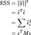
Estimation of ![]() is based on the error sum of squares defined by
is based on the error sum of squares defined by

where
![]()
We compute the mean of ESS as follows:
![\begin{align*}{\rm E}[{\rm ESS}] & =
{\rm E}(\epsilon^T M \epsilon)
\\
& = {\rm...
...\sigma^2 I)
\\
& = \sigma^2 {\rm trace}(M)
\\
& = \sigma^2 ( n-p)
\end{align*}](img5.gif)
So:

is an unbiased estimate of ![]() .
.
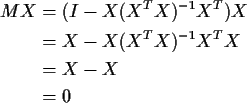
FACT: Every Sum of Squares we will see is of the form
FACT: Often we find
Example:

So we find

Messages to take away from this example:
We will follow up these points later. Now we turn to the third application of matrix algebra mentioned in lecture 9.
Examples of linear combinations:
Basic Ingredients:


We have done the mathematics for 1, 2 ,4, 5 above. Fact number 8 is just the definition of the Student t distribution together with facts 5, 6 and 7. Fact number 9 is just the usual deduction of a confidence from the distribution of a pivot as in 8. I will wave my hands at the mathematics of 6 and 7 later in the course.
Refer to the polynomial regression example (data on insurance
costs). Suppose we are going to use a polynomial model of degree p and
try to predict the costs for the first quarter of 1982, that is, for
t=1982.25. Our model has
![\begin{align*}\hat\mu_{1982.25} & = \hat\beta_0 + \hat\beta_1(1982.25-1975.5) + ...
...n{array}{c} \hat\beta_0 \\ \vdots \\ \hat\beta_p\end{array} \right]
\end{align*}](img30.gif)
Our confidence interval for the expected cost for 1982.25 is

Here is a table of the computed confidence intervals:
| Degree p | t |
|
||
| 1 | 113.98 | 2.306 | 7.04 | 16.24 |
| 2 | 142.04 | 2.365 | 12.06 | 28.53 |
| 3 | 204.74 | 2.447 | 9.45 | 23.12 |
| 4 | 204.50 | 2.571 | 25.24 | 64.88 |
| 5 | 70.26 | 2.776 | 16.22 | 16.22 |
Notice that the forecasts for different polynomials are very diffferent and not within several standard errors of each other.
Problem: Let ![]() be the true mean of Yx.
Our MODEL says that
be the true mean of Yx.
Our MODEL says that
![]() but most or all of
these polynomials are WRONG.
but most or all of
these polynomials are WRONG.
You can see the principal by deleting the observation for 1980, then fitting the different polynomials, and predicting the 1980 value:
| Degree | Estimate | SE |
| p | for 1980 | of estimate |
| 1 | 91.50 | 4.26 |
| 2 | 98.22 | 7.34 |
| 3 | 121.39 | 4.74 |
| 4 | 132.40 | 6.73 |
| 5 | 110.40 | 4.59 |
The calculations given above provide confidence intervals for the
expected value of Y for 1982.25. In fact each Y differs from
its expected value by a random ![]() .
Thus the figure of $115.19
is not realy
.
Thus the figure of $115.19
is not realy
![]() bu Y1980.
bu Y1980.
To predict an observation, however, we guess
![]() by guessing
by guessing
![]() and adding a guess for
and adding a guess for ![]() .
Since
.
Since ![]() is a mean 0
random variable, independent of all the other random variables used to
predict
is a mean 0
random variable, independent of all the other random variables used to
predict ![]() we simply guess
we simply guess ![]() is 0 and use
is 0 and use
![]() .
But then
.
But then

We call the square root of this quantity the root mean square
, or RMS, Prediction Error and estimate this RMS prediciton
error using
| Degree |
|
RMS Pred Err |
| 1 | 42.6 | 7.25 |
| 3 | 4.74 | 5.22 |
| 5 | 4.59 | 4.63 |
The general formula for a level ![]() prediction interval for
Yx is
prediction interval for
Yx is
I fit polynomials of degree 1 through 5. Each model gives
a vector of fitted parameters ![]() and to predict the mean value
of Y at time t we use
and to predict the mean value
of Y at time t we use
![]() when the fitted polynomial has degree p. The
SAS code below computes both this fitted value and standard errors
for each of the 5 models. Notice how I run proc glm 5 times
to get the 5 different values.
when the fitted polynomial has degree p. The
SAS code below computes both this fitted value and standard errors
for each of the 5 models. Notice how I run proc glm 5 times
to get the 5 different values.
data insure;
  infile 'insure.dat' firstobs=2;
  input year cost;
  code = year - 1975.5 ;
proc glm  data=insure;
   model cost = code ;
   estimate 'fit1982.25' intercept 1 code  6.75  / E;
run ;
proc glm  data=insure;
   model cost = code code*code;
   estimate 'fit1982.25' intercept 1 code  6.75 code*code 45.5625 / E;
run ;
proc glm  data=insure;
   model cost = code code*code code*code*code;
   estimate 'fit1982.25' intercept 1 code  6.75 code*code
            45.5625 code*code*code 307.5469/ E;
run ;
proc glm  data=insure;
   model cost = code code*code code*code*code code*code*code*code;
   estimate 'fit1982.25' intercept 1 code  6.75 code*code
            45.5625 code*code*code 307.5469 code*code*code*code
            2075.9414 / E;
run ;
proc glm  data=insure;
   model cost = code code*code code*code*code code*code*code*code
                code*code*code*code*code;
   estimate 'fit1982.25' intercept 1 code  6.75 code*code
            45.5625 code*code*code 307.5469 code*code*code*code
            2075.9414 code*code*code*code*code 14012.6045/ E;
run ;
The line estimate ... is probably unfamiliar to you. You have to
give the values of each column of the design matrix at the place where you
want to estimate Now have a look at the edited output. I show here only the 5th degree polynomial results.
                        General Linear Models Procedure
Coefficients for estimate fit1982.25
INTERCEPT                                         1
CODE                                           6.75
CODE*CODE                                   45.5625
CODE*CODE*CODE                             307.5469
CODE*CODE*CODE*CODE                       2075.9414
COD*COD*COD*COD*CODE                     14012.6045

Dependent Variable: COST
                                     Sum of            Mean
Source              DF          Squares          Square   F Value     Pr > F

Model                5     3935.2507732     787.0501546   2147.50     0.0001
Error                4        1.4659868       0.3664967
Corrected Total      9     3936.7167600

              R-Square             C.V.        Root MSE            COST Mean
              0.999628         0.851438       0.6053897            71.102000

Source              DF        Type I SS     Mean Square   F Value     Pr > F
CODE                 1     3328.3209709    3328.3209709   9081.45     0.0001
CODE*CODE            1      298.6522917     298.6522917    814.88     0.0001
CODE*CODE*CODE       1      278.9323940     278.9323940    761.08     0.0001
CODE*CODE*CODE*CODE  1        0.0006756       0.0006756      0.00     0.9678
COD*COD*COD*COD*CODE 1       29.3444412      29.3444412     80.07     0.0009

Source              DF      Type III SS     Mean Square   F Value     Pr > F
CODE                 1       0.88117350      0.88117350      2.40     0.1959
CODE*CODE            1      20.86853994     20.86853994     56.94     0.0017
CODE*CODE*CODE       1      72.35876312     72.35876312    197.43     0.0001
CODE*CODE*CODE*CODE  1       0.00067556      0.00067556      0.00     0.9678
COD*COD*COD*COD*CODE 1      29.34444115     29.34444115     80.07     0.0009

                                    T for H0:    Pr > |T|   Std Error of
Parameter              Estimate    Parameter=0                Estimate
fit1982.25           70.2630583           4.33     0.0123     16.2154539

                                     T for H0:    Pr > |T|   Std Error of
Parameter               Estimate    Parameter=0                Estimate

INTERCEPT            64.88753906         176.14     0.0001     0.36839358
CODE                 -0.50238411          -1.55     0.1959     0.32399642
CODE*CODE             0.75623470           7.55     0.0017     0.10021797
CODE*CODE*CODE        0.80157430          14.05     0.0001     0.05704706
CODE*CODE*CODE*CODE  -0.00020251          -0.04     0.9678     0.00471673
COD*COD*COD*COD*CODE -0.01939615          -8.95     0.0009     0.00216764
While we have this output notice the value of R2 which is quite close to 1 and the t-tests of hypotheses that various parameters are 0.
Here is a table of the results of all the forecasts with associated standard errors:
| Degree | Estimate | SE |
1 |
113.98 | 7.04 |
| 2 | 142.04 | 12.06 |
| 3 | 204.74 | 9.45 |
| 4 | 204.50 | 25.24 |
| 5 | 70.26 | 16.22 |
One final point. The calculations give a confidence interval
for ![]() based on the distribution of
based on the distribution of
![]() .
For
the insurance the quantity of interest is
.
For
the insurance the quantity of interest is
![]() .
In this formula, Yx is a future value associated with the covariate
value x. The prediction can be split up, if the model is correct, as
.
In this formula, Yx is a future value associated with the covariate
value x. The prediction can be split up, if the model is correct, as
You can see the principal by deleting the observation for 1980 and then fitting the different polynomials:
| Degree | Estimate | SE of |
Prediction SE |
| 1 | 91.50 | 4.26 | 7.25 |
| 2 | 98.22 | 7.34 | 9.34 |
| 3 | 121.39 | 4.74 | 5.22 |
| 4 | 132.40 | 6.73 | 6.95 |
| 5 | 110.40 | 4.59 | 4.63 |