Reading: Chapter 6.1-6.
Assume:
Define: H= X(XT X)-1 XT, the hat matrix so that M=I-H.
If also
If also
![]() are independent then
are independent then
Notice
![]() and that H is
and that H is
![]() .
.
Some algebraic simplification of the variances above is possible.

But
![\begin{align*}H^T & = \left[ X(X^T X)^{-1} X^T\right]^T
\\
& = X\left[(X^T X)^{...
...X)^T\right]^{-1} X^T
\\
&= X \left[ X^TX\right]^{-1} X^T
\\
& = H
\end{align*}](img16.gif)
ASIDE: as you read that sequence of formulas you will see that I expect you to remember a number of algebraic facts about matrices:
So

Thus

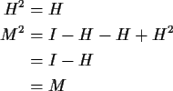
Definition: A matrix Q is idempotent if
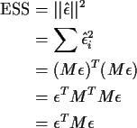
Estimation of ![]() is based on the error sum of squares defined by
is based on the error sum of squares defined by

Now note that
![\begin{align*}{\rm E}[{\rm ESS}] & =
{\rm E}(\epsilon^T M \epsilon)
\\
& = {\rm...
...\epsilon_j]
\\
& = \sum_{ij} M_{ij} {\rm E}[\epsilon_i \epsilon_j]
\end{align*}](img25.gif)
But
![]() for
for ![]() and
and
![]() so
so
![\begin{align*}{\rm E}[{\rm ESS}] & = \sigma^2 \sum_i M_{ii}
\\
& = \sigma^2 {\rm trace}(M)
\end{align*}](img29.gif)
Definition: The trace of a square matrix Q is defined by

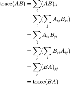
Marvelous Matrix Identity (cyclic invariance of the trace).
Suppose that
![]() and
and
![]() so that
so that
![]() and
and
![]() are both square. Then
are both square. Then

The same idea works with more than two matrices provided the product is
square so, e.g.,
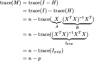
Another algebraic identity for the trace:

SO:

Notice that p is the number of columns of X including the column of 1's if present.
![\begin{displaymath}{\rm E}\left[ \frac{{\rm ESS}}{n-p}\right] = \sigma^2
\end{displaymath}](img39.gif)
So the Mean Squared Error, ESS/(n-p) is an unbiased estimate of
![]() .
.
Here is an example of some of the matrix algebra I was doing in class.
Consider the weighing design where two objects of weights ![]() and
and
![]() are weighed individually and together. The resulting design
matrix is
are weighed individually and together. The resulting design
matrix is
![\begin{displaymath}X = \left[\begin{array}{rr} 1 & 0 \\ 0 & 1 \\ 1 & 1\end{array}\right]
\end{displaymath}](img42.gif)
So
![\begin{displaymath}X^tX = \left[\begin{array}{rr} 2 & 1 \\ 1 & 2 \end{array}\right]
\end{displaymath}](img43.gif)
![\begin{displaymath}(X^TX)^{-1} = \left[\begin{array}{rr} \frac{2}{3} & -\frac{1}{3} \\
-\frac{1}{3} & \frac{2}{3} \end{array}\right]
\end{displaymath}](img44.gif)
The hat matrix is
![\begin{displaymath}\left[\begin{array}{rr} 1 & 0 \\
0 & 1 \\ 1 & 1\end{array}\r...
...[\begin{array}{rrr}
1 & 0 & 1 \\ 0 & 1 & 1 \end{array}\right]
\end{displaymath}](img45.gif)
![\begin{displaymath}\left[\begin{array}{rrr}
\frac{2}{3} & -\frac{1}{3} & \frac{1...
...\
\frac{1}{3} & \frac{1}{3} & \frac{2}{3}
\end{array}\right]
\end{displaymath}](img46.gif)
You can also check that H is idempotent.