Reading: Chapter 5, chapter 15.
So far we have defined:

![\begin{displaymath}Z = \left[ \begin{array}{c} Z_1 \\ \vdots \\ Z_n \end{array} \right] \sim
MVN_n(0,I)
\end{displaymath}](img5.gif)
![\begin{displaymath}\mu_X \equiv {\rm E}\left(
\left[\begin{array}{c} X_1 \\ \vdo...
...array}{c} E(X_1) \\ \vdots \\ {\rm E}(X_n) \end{array} \right]
\end{displaymath}](img6.gif)
![\begin{displaymath}{\rm E} \left[
\begin{array}{ccc}
M_{11} & \cdots & M_{1c}
\...
...
{\rm E}(M_{r1}) & \cdots & {\rm E}(M_{rc})
\end{array}\right]
\end{displaymath}](img7.gif)
Now suppose
![]() .
Then
.
Then
![\begin{displaymath}{\rm E}(Z) = \left[ \begin{array}{c}
{\rm E}(Z_1) \\ \vdots \\ {\rm E}(Z_n)
\end{array}\right]
= {\bf0}_n
\end{displaymath}](img14.gif)
Next we compute the variance of Z. Note that
![]() has ijth entry
has ijth entry

So
Now suppose that
Now
![]() has ith component
has ith component
![\begin{align*}{\rm E}[(AZ)_i] + \mu_i
& = {\rm E}( \sum_j A_{ij} Z_j) + \mu_i
\\
& = \sum_j A_{ij} {\rm E}(Z_j) + \mu_i
\\
& = \mu_i
\end{align*}](img26.gif)
Moreover,
![\begin{align*}{\rm Var}(X) & = {\rm E}(\left[ (X-\mu)(X-\mu)^T \right]
\\
& = {...
...m E}[AZZ^T A^T]
\\
& = A {\rm E}[ZZ^T] A^T
\\
& = AIA^T
\\
=AA^T
\end{align*}](img27.gif)
The last three lines need some justification. The point is that
matrix multiplication by A, whose entries are constants,
is just like multiplication by a constant -- you can pull the
constant outside of the expected value sign. Here is the justification.
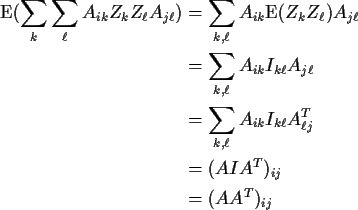
The ijth entry in
![]() is
is

So,
![]() .
.
Thus
![]() means that
means that
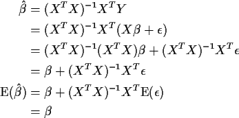
The following do not use the normal assumption:

So ![]() is unbiased.
is unbiased.

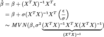
If, also,
![]() then
then
![]() and
and

The fitted vector is
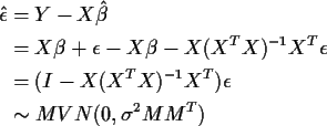
The residual vector is

where
M=I-X(XT X)-1 XT).
Notation:
Jargon: H is called the hat matrix. Notice that
I tried, as I was calculating things for the vectors ![]() ,
,
![]() and
and
![]() to emphasize which things needed which
assumptions.
to emphasize which things needed which
assumptions.
So for instance we have following matrix identities which depend
only on the model equation
If we add the assumption that
![]() for each i then we get
for each i then we get
If we add the assumption that the errors are homoscedastic
(
![]() for all i) and uncorrelated
(
for all i) and uncorrelated
(
![]() for all
for all ![]() )
then we can compute variances and get
)
then we can compute variances and get
NOTE: usually we assume that the
![]() are independent and
identically distributed which guarantees the homoscedastic, uncorrelated
assumption above.
are independent and
identically distributed which guarantees the homoscedastic, uncorrelated
assumption above.
Next we add the assumption that the errors
![]() are independent
normal variables. Then we conclude that each of
are independent
normal variables. Then we conclude that each of ![]() ,
,
![]() and
and
![]() have Multivariate Normal distributions with the means and
variances as just described.
have Multivariate Normal distributions with the means and
variances as just described.