Reading: 6.5, Chapter 15, Appendix A.
An informal method of selecting p, the model order, is based on

Note: adding more terms always increases R2.
Formal methods can be based on hypothesis tests. We can
test
![]() and then, if we accept this test
and then, if we accept this test
![]() and then, if we accept that test
and then, if we accept that test
![]() and so on stopping when we first reject a hypothesis. This is
``backwards elimination''.
and so on stopping when we first reject a hypothesis. This is
``backwards elimination''.
Justification: Unless ![]() there is no good reason to
suppose that
there is no good reason to
suppose that ![]() and so on.
and so on.
Apparent conclusion in our example: p=5 is best; look at the P values in the SAS outputs.
Problems arising with that conclusion:
Question: What is distribution theory?
Answer: How to compute the ``distribution'' of an estimator, test or other statistic, T:
In this course we
The standard normal density is


Reminder: if X has density f(x) then

So:
![]() implies
implies


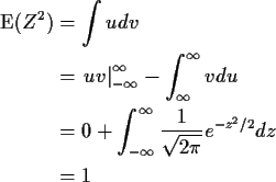
Next we compute the variance of Z remembering that
![]() :
:

where
![]() and
dv = -ze-z2/2 dz. We do integration
by parts and see that
v=e-z2/2 and
and
dv = -ze-z2/2 dz. We do integration
by parts and see that
v=e-z2/2 and
![]() .
This gives
.
This gives

because the integral of the normal density is 1. We have thus shown
that
Definition: If
![]() then
then
![]() .
.
Note:

Definition: If
![]() are independent N(0,1)
then
are independent N(0,1)
then
![\begin{displaymath}Z = \left[ \begin{array}{c} Z_1 \\ \vdots \\ Z_n \end{array} \right] \sim
MVN(0,I)
\end{displaymath}](img31.gif)
We can define
![]() and
and
![]() for vectors like Z as
follows:
for vectors like Z as
follows:
If X is a random vector of length n, say
![]() then
then
![\begin{displaymath}\mu_X \equiv {\rm E}(X) = \left[
\begin{array}{c} {\rm E}(X_1) \\ \vdots \\ {\rm E}(X_n) \end{array} \right]
\end{displaymath}](img35.gif)
Definition:
![\begin{align*}{\rm Cov}(X_i,X_j) & = {\rm E} \left[
(X_i - {\rm E}(X_i))(X_j-{\r...
...m E}(X_j)\right]
\\
&= {\rm E}(X_i X_j) - {\rm E}(X_i){\rm E}(X_j)
\end{align*}](img41.gif)
Definition: If M is a matrix then
![]() is a matrix
whose ijth entry is
is a matrix
whose ijth entry is
![]() .
.
So
![]() has ijth entry
has ijth entry
![]() and
diagonal entries
and
diagonal entries
![]() .
.
In class I started discussion of the Normal distribution. I computed the
mean and variance of a standard normal and then of
![]() .
Here I will just show you a few more integrals:
.
Here I will just show you a few more integrals:
The kth moment of a standard normal is


We can also compute the moment generating function of Z, that is,


Now if
![]() then
then
![]() so
that the
so
that the
![]() central moment of X, namely
central moment of X, namely
![]() is 0 for odd k and
is 0 for odd k and
![]() for k even.
for k even.
Similarly