 are independent random variables each having a
 distribution. Let
 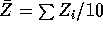 ,
, 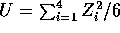 ,
,
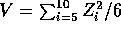 ,
, 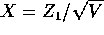 and
and  .
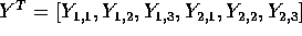
Give the names for the distributions of each of
.
Give the names for the distributions of each of  , U, V, X and Y
and use tables to find
, U, V, X and Y
and use tables to find  ,
,  ,
,  ,
,
 ,
,  ,
,  .
.
 is
is  , U is
  , V is
  , X is
  ,
since
,
since  and V are independent and
 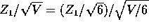 , and
, and 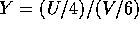 has an
  distribution, using the fact that U and V are independent. Your answer
should specify the mean and variance for
distribution, using the fact that U and V are independent. Your answer
should specify the mean and variance for  , the various degrees of
freedom and note the required independence for X and Y.
The required probabilities are 0.197, 0.05, 0.725, 0.025, 0.688, 0.034.
I used SPlus to compute these; if you used tables your answers will be less
accurate.
, the various degrees of
freedom and note the required independence for X and Y.
The required probabilities are 0.197, 0.05, 0.725, 0.025, 0.688, 0.034.
I used SPlus to compute these; if you used tables your answers will be less
accurate.
 for
for  ;
the new process is used to measure the concentrations for these samples.
It is thought likely that the concentrations measured by the new process,
which we denote
;
the new process is used to measure the concentrations for these samples.
It is thought likely that the concentrations measured by the new process,
which we denote  , will be related to the true concentrations via

where the  are independent, have mean 0 and all have the
same variance
are independent, have mean 0 and all have the
same variance  which is unknown.
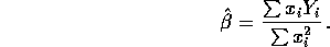
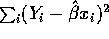
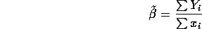
- If this model is fitted by least squares, (that is by minimizing
 ) show that the least squares estimate of
 is
is
Differentiate
 with respect to
  and
get
and
get 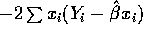 which is 0 if and only if
 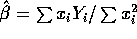 . The second derivative of the function being
minimized is
. The second derivative of the function being
minimized is  so this is a minimum.
- Show that the estimator in part (a) is unbiased.
Let
 . Then
 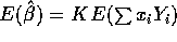 . Use
. Use
 to see that
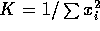
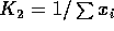
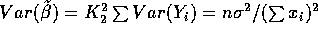
- Compute (give a formula for) the standard error of
 .
.
You have to compute
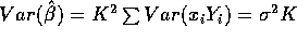 which is simply
  .
.
- The error sum of squares for this model is
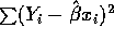 which may be shown to have n-1 degrees of freedom.
If the
which may be shown to have n-1 degrees of freedom.
If the  are the numbers 1, 2, 3 and 4,
  and the
error sum of squares is 0.12 find a 95% confidence interval for
and the
error sum of squares is 0.12 find a 95% confidence interval for  and explain what further assumptions you must make to do so.
If we assume that the errors are independent
 ) random
variables then
) random
variables then  is independent of the usual estimate of
 , samely
 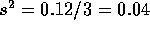 in this case. The usual t
statistic then has a t distribution and the confidence interval
is
in this case. The usual t
statistic then has a t distribution and the confidence interval
is 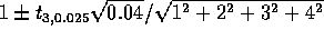 which boils down to
 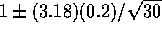 .
.
- Show that the estimator
is also unbiased.
Let
 ; then
 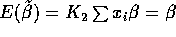 .
.
- Compute (give a formula for) the standard error of
 . Which
is bigger, the standard error of
. Which
is bigger, the standard error of  or that of
  ?
?
We have
 .
The difference
.
The difference 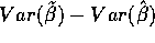 is then simply
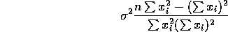
The denominator is positive and the numerator is
 times the usual
sample variance of the x's so this difference of variances is positive.
times the usual
sample variance of the x's so this difference of variances is positive.
- Show that the mle of
 in this model is
  , the least
squares estimate, if the
, the least
squares estimate, if the  have normal distributions.
In this case
 is
is  and the likelihood is

As usual you maximize the logarithm which is

Take the
 derivative and get the same equation to solve for
  as in the first part of this problem.
 for
for
 and
and  . We generally fit a so-called additive model

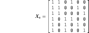
In the following questions consider the case I=2 and J=3.
- If we treat
 ,
,  ,
,  ,
,  ,
,  and
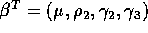
and  as the entries in the parameter vector
  what is the design matrix
  and what
is the rank of
and what
is the rank of  ?
?
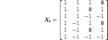
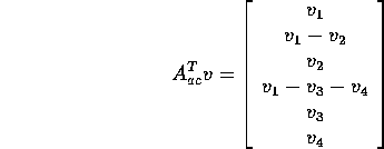
Writing the data as
 the design matrix is
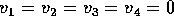
Letting
 denote column i of
  we have
  and
and  so that the rank of
  must be no more than
4. But if
must be no more than
4. But if  then from row 6
we get
then from row 6
we get  . Then from rows 4 and 5 get
  and
and  . Finally use
row 3 to get
. Finally use
row 3 to get  . This shows that columns 1, 2 4 and 5 are linearly
independent so tha t
. This shows that columns 1, 2 4 and 5 are linearly
independent so tha t has rank at least 4 and so exactly 4.
- What is the determinant of the matrix
 ? Is this matrix invertible? How many
solutions do the normal equations have?
? Is this matrix invertible? How many
solutions do the normal equations have?
The matrix
 is 6 by 6 but has rank only 4 so is singular and
must have determinant 0. The normal equations are
is 6 by 6 but has rank only 4 so is singular and
must have determinant 0. The normal equations are
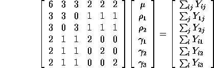
It may be seen that the second and third rows give equations which add up to the equation in the first row as do the fourth, fifth and sixth rows. Eliminate rows 3 and 6, say and solve. This leaves 4 linearly independent equations in 6 unknowns and so there are infinitely many solutions.
- Usually we impose the restrictions
 and
and 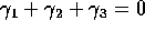 .
Use these restrictions to eliminate
.
Use these restrictions to eliminate  and
and  from the model equation
and, for the parameter vector
from the model equation
and, for the parameter vector 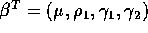 find the design
matrix
find the design
matrix  .
.
The restrictions give
 and
and 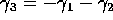 . In each model equation which mentions either
  or
or
 you replace that parameter by the equivalent formula. So, for
example,
you replace that parameter by the equivalent formula. So, for
example,

The 6th row of the design matrix is obtained by reading off the coefficients of
 which are 1, -1, -1 and
-1. This makes
which are 1, -1, -1 and
-1. This makes
- An alternate set of restrictions is called corner point coding where we assume
 . With this restriction and the parameter vector
 what is the design matrix
  ?
?
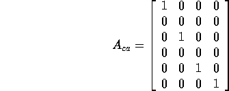
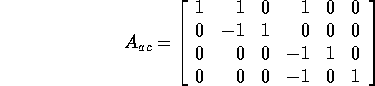
This just makes the design matrix
 just the corresponding columns, 1, 3, 5
and 6 of
just the corresponding columns, 1, 3, 5
and 6 of  .
.
- Show that the three design matrices have the same column space by finding a matrix
A such that
 and similarly for
  and
and  and for
  and
and  .
.
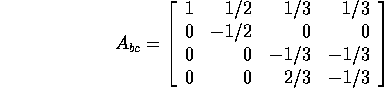
To write
 just let A be the
  matrix which picks
out columns 1,3,5 and 6 of
matrix which picks
out columns 1,3,5 and 6 of  , namely,
To write
 we just have to put back column 2 and 4 remembering that
col 2 is col 1 - col 3 and col 4 is col 1 - col 5 - col 6. Thus
we just have to put back column 2 and 4 remembering that
col 2 is col 1 - col 3 and col 4 is col 1 - col 5 - col 6. Thus
Similarly
A vector in the column space of say
 is of the form
  for a vector of
coefficients v. But such a vector is
for a vector of
coefficients v. But such a vector is  and so of the form
  for the vector
  and so in the column space of
  .
.
- Use the previous part to show that the vectors of fitted values
 will be the
same for any solution of the normal equations for any of the three design matrices.
will be the
same for any solution of the normal equations for any of the three design matrices.
The easy way to do this is to say: the fitted vector
 is the closest point
in the column space of the design matrix to the data vector Y. Since all three have the
same column space they all have the same closest point and so the same
is the closest point
in the column space of the design matrix to the data vector Y. Since all three have the
same column space they all have the same closest point and so the same  .
.
Algebra is an alternative tactic: The matrix
 is invertible and we have

Plug in
 for
for  and get

Use
 to see that all occurences of
  cancel
out to give
cancel
out to give

The algebraic approach makes it a bit more difficult to deal with the case of
 because the normal equations have many solutions.
Suppose that
because the normal equations have many solutions.
Suppose that  is any solutions of the normal equations
 . Then

The matrix
 has rank 4. If any vector v satisfies
  then
then
so that
 . This shows that

so that
 .
.
Thus

Postponed to next assignment.